Recreating analyses from the CRUX manuscript
This appendix demonstrates how to perform each analysis from the manuscript:
CRUX, a platform for visualising, exploring and analysing cancer genome cohort data, by El-Kamand et al.
Please cite the above publication and the authors of any external tools accessed using CRUX.
Short study 1: Driver Identification
Identify putative driver oncogenes from glioblastoma multiforme (GBM) tumours.
A video tutorial recreating this study is available here
Short study 2: Prognostic Biomarkers
Identify biomarkers associated with patient survival by integrating genome molecular alterations with clinical data.
Dataset: The inbuilt GBM cohort dataset (n = 283) from TCGA, as in short study 1.
Here we study how patient survival in the GBM cohort relates to mutations in genes of interest. The first step is to access the Survival Analysis page, which is available under the Single Cohort Genomics menu on the Crux sidebar [screenshot 1].
Screenshot 1
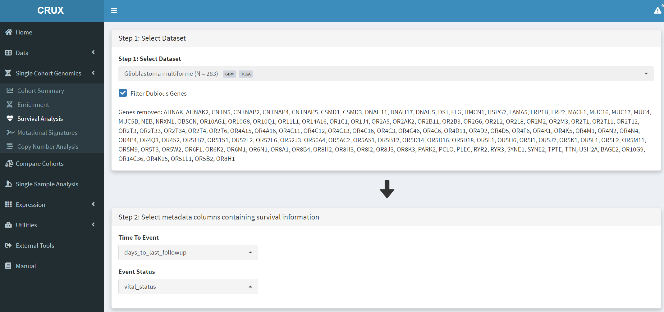
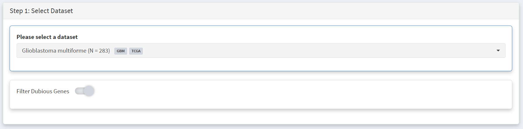
On this page the GBM dataset is selected and loaded. In the Step 1 panel, ‘glioblastoma’ is searched in the selection field and the Glioblastoma multiforme dataset is then selected. The Filter Dubious Genes option is also selected on that panel.
In the Step 2 panel the Time To Event dropdown menu is selected and option ‘days_to_last_followup’ chosen. From the Event Status dropdown menu ‘vital_status’ option is chosen. These two options delineate the time to event needed to perform survival analysis on this GBM dataset.
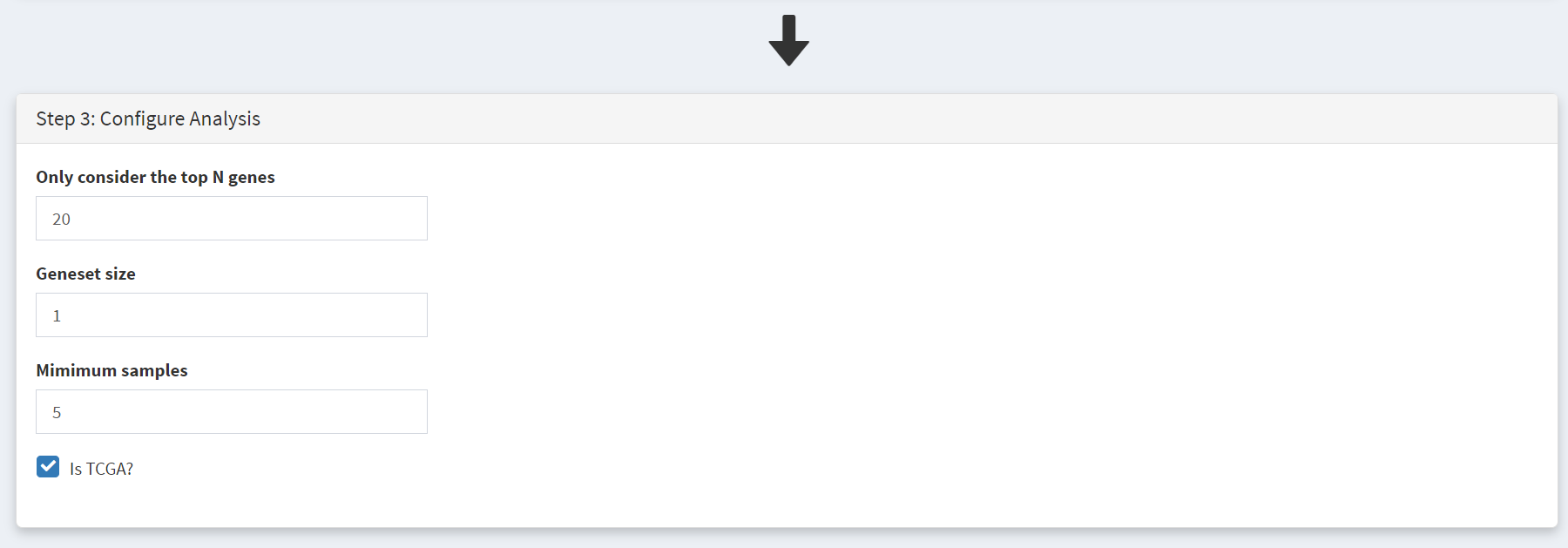
Further filtering of the geneset can be performed on Step 3 panel [screenshot 2], changing these filter values can greatly affect the output table:
’Only consider the top N genes’ filter - genes are ranked by number of samples bearing mutations in them, and removes all genes outside the top N highly ranked genes. The effect of mutations in each of the top N genes on patient survival are examined. Note that the table below does not use this ranking as it ranks by hazard ratio p-value.
‘Geneset size’ filter – setting this to 1 (default) looks at genes individually, while setting to 2 means that pairs of genes are examined, so that samples with mutations in a pair of 2 genes (such as TP53 and RB1) for an effect on patient survival.
‘Minimum size’ filter – excluded genes that show mutations in fewer than this number of samples.
Changing these filters can greatly alter the genes included in the table in screenshot 3. It is also important to remove genes with many passenger mutations using the filter dubious genes button.
Screenshot 2
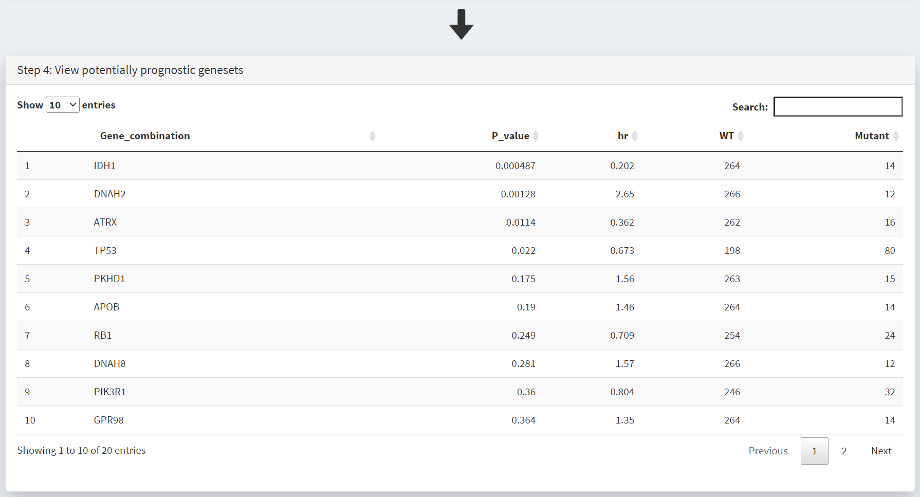
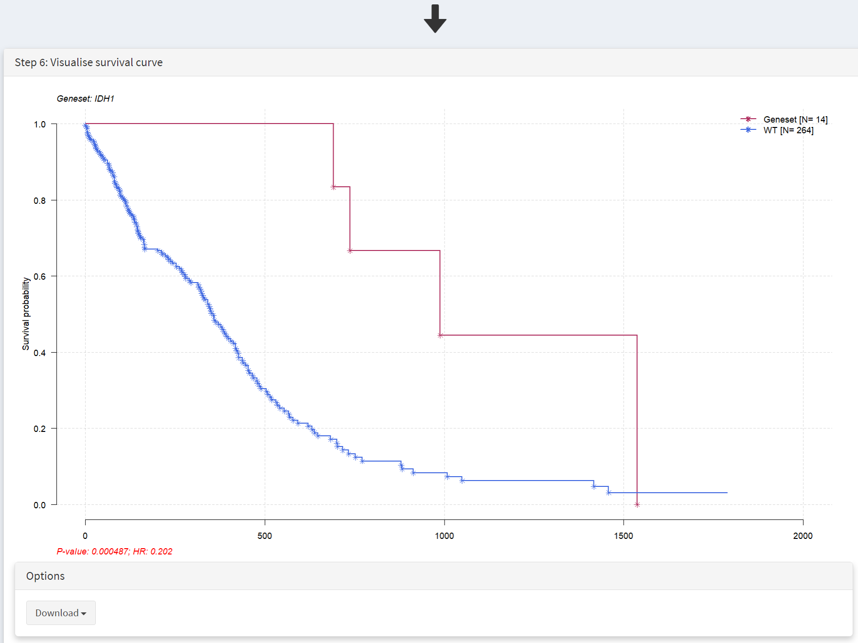
This populates the Step 4 panel with a list of genes ordered by the p-value of the survival hazard ratio, comparing survival of patients that have mutations in a specific gene with patients that do not. Screenshot 3 shows the data for from the top 10 genes in GBM, with IDH1 mutations (p-value of 0.000487) at the top of the list. The hazard ratio of 0.202 is well below 1, indicating much better survival of these patients than those without IDH1 mutations. Note that only 14 patients have IDH1 mutations. None of the genes beyond TP53 show p-value less than 0.05.
Screenshot 3
Warning
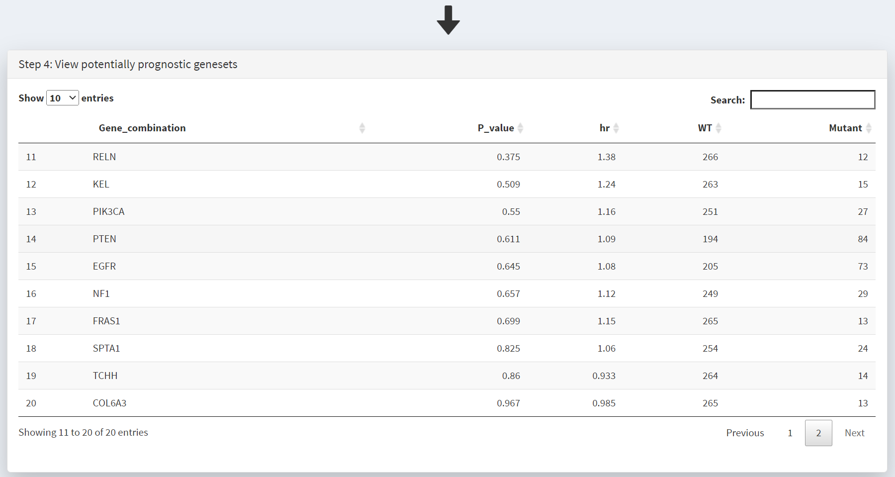
The P values displayed above are not adjusted for multiple testing. Depending on how you present these findings, you may need to correct for the total number of ‘tests’ (number of different genes/genesets examined. In this example there are ‘20’ genes in the table, as indicated by the caption ‘Showing 1 to 10 of [20] entries’
Screenshot 4 shows the next 10 genes on this list; the top 20 genes were selected. Note that in the CRUX manuscript (Fig. 3) the gene STAG2 was included in the table as the top N gene filter was set to 40, and STAG2 is mutated in only 12 samples; this is an example of the effects of changing this filter number.
Screenshot 4
Plotting of survival information for a gene is performed on the Step 5 panel. To examine IDH1 mutations this gene is selected under the Select Genest menu [screenshot 5].
Screenshot 5
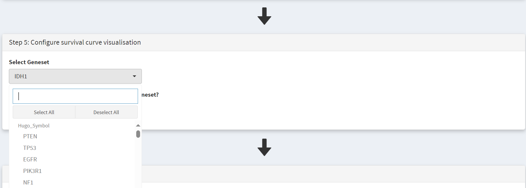
This selection produces a Kaplan Meier plot in the Step 6 Visualisation panel [screenshot 6]. Note that the gene (or genes) selected are labelled as ‘Geneset’ and are compared to ‘WT’, i.e., no mutation. More than one gene can be selected so that the effects of gene mutation combinations can be explored.
Screenshot 6
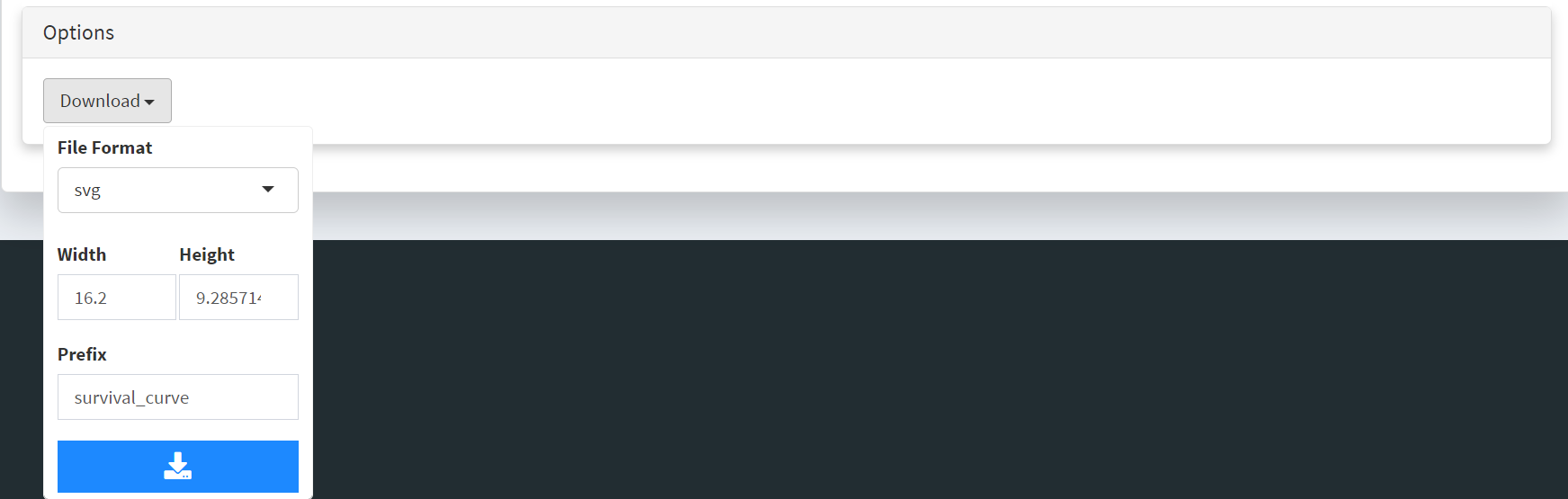
This plot can be downloaded for use using the Download button as seen in [screenshot 7].
Screenshot 7
Next to identify the mutations of interest we move to the Lollipop tab (Single Cohort Genomics > Cohort Summary) and select the GBM dataset, as shown in [screenshot 8].
Screenshot 8
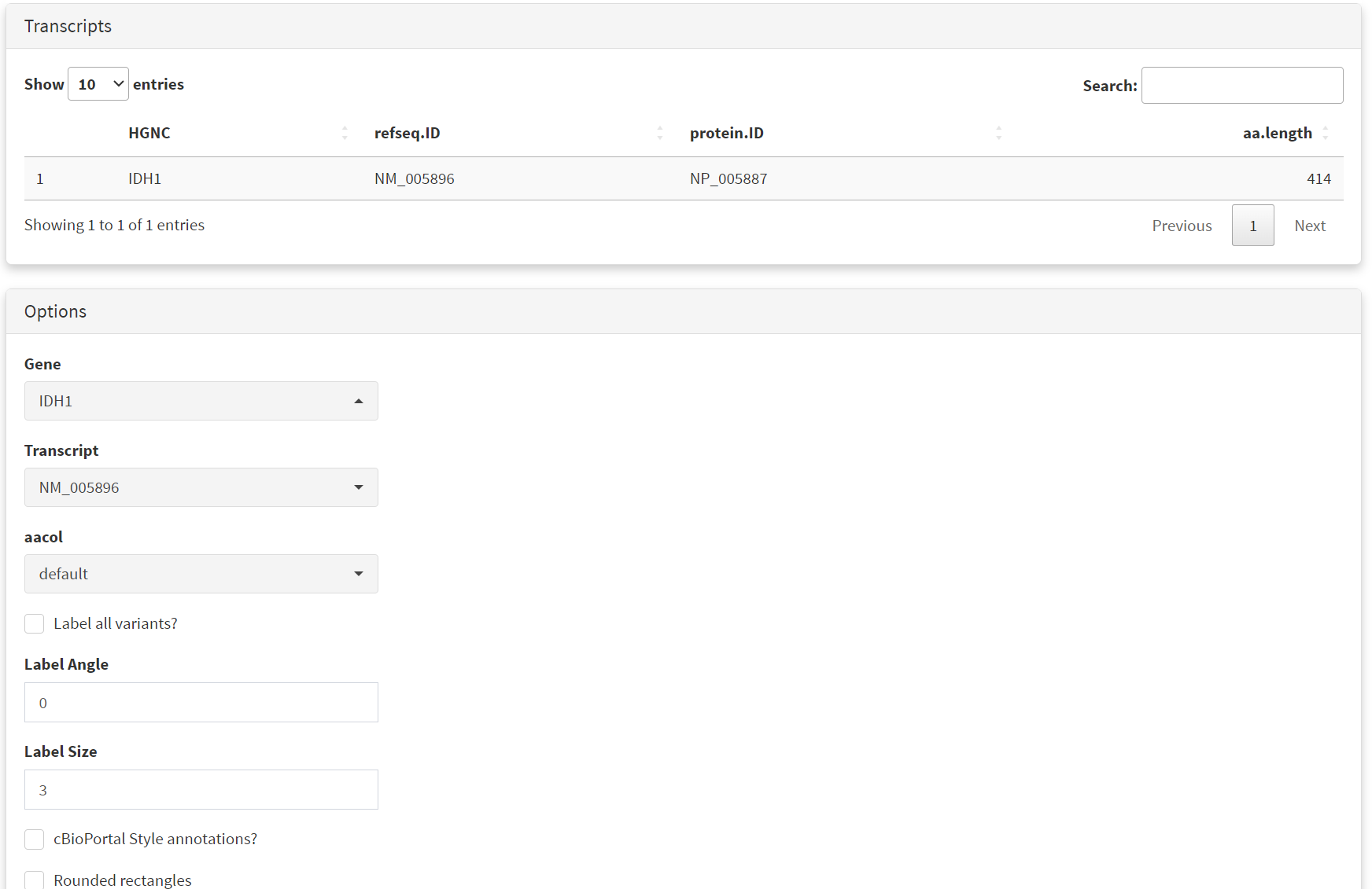
This gives the Lollipop plot for the selected gene. Screenshot 9 shows the Lollipop tab of the Step 2 panel, which indicates recurrance and position of all mutations GBM mutations in a user-specified protein (and defined protein domains). Here IDH1 was selected in the lower part of the panel under the Gene menu [screenshot 10]. For this gene it is notable that all mutations in the cohort occur at one site corresponding to amino acid 132.
Screenshot 9

Screenshot 10
Short study 3: Therapeutic Relevance of Driver Mutations
Identification of candidate driver mutations linked to therapeutic responses in thyroid cancer.
Note
Only a subset of the analyses described below were included Figure 4 of the El-Kamand et al.
Dataset: The inbuilt TCGA Thyroid Cancer (THCA) dataset, generated from whole exome sequencing of 496 patient samples.
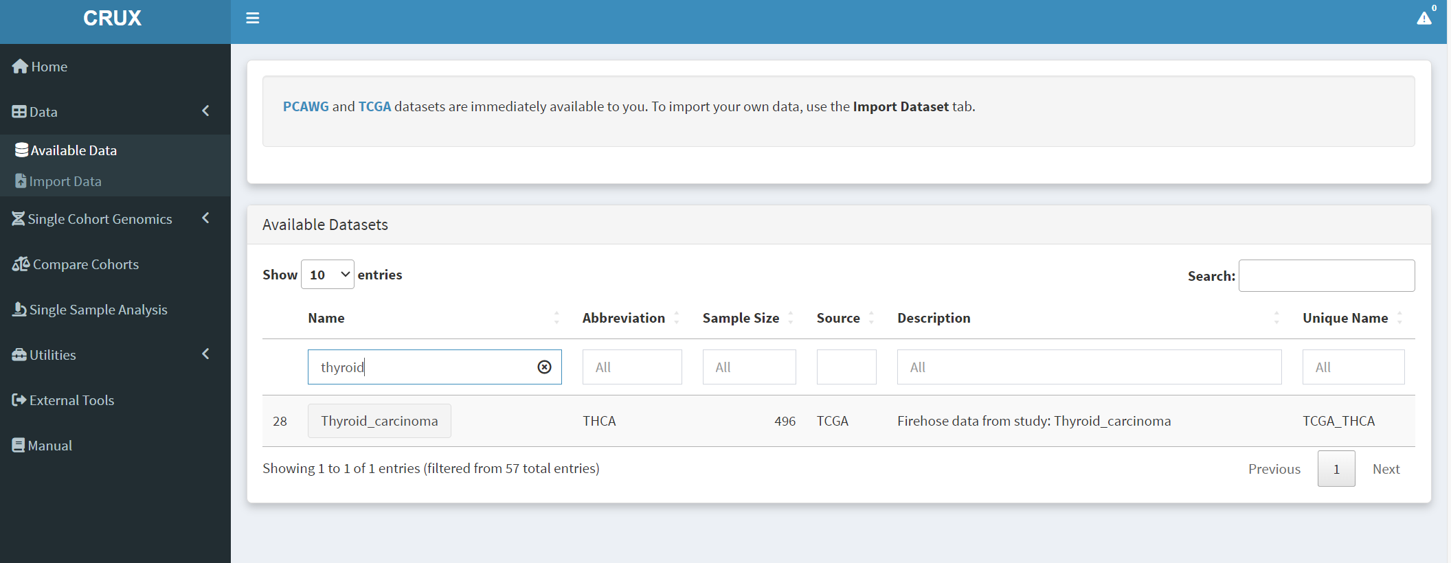
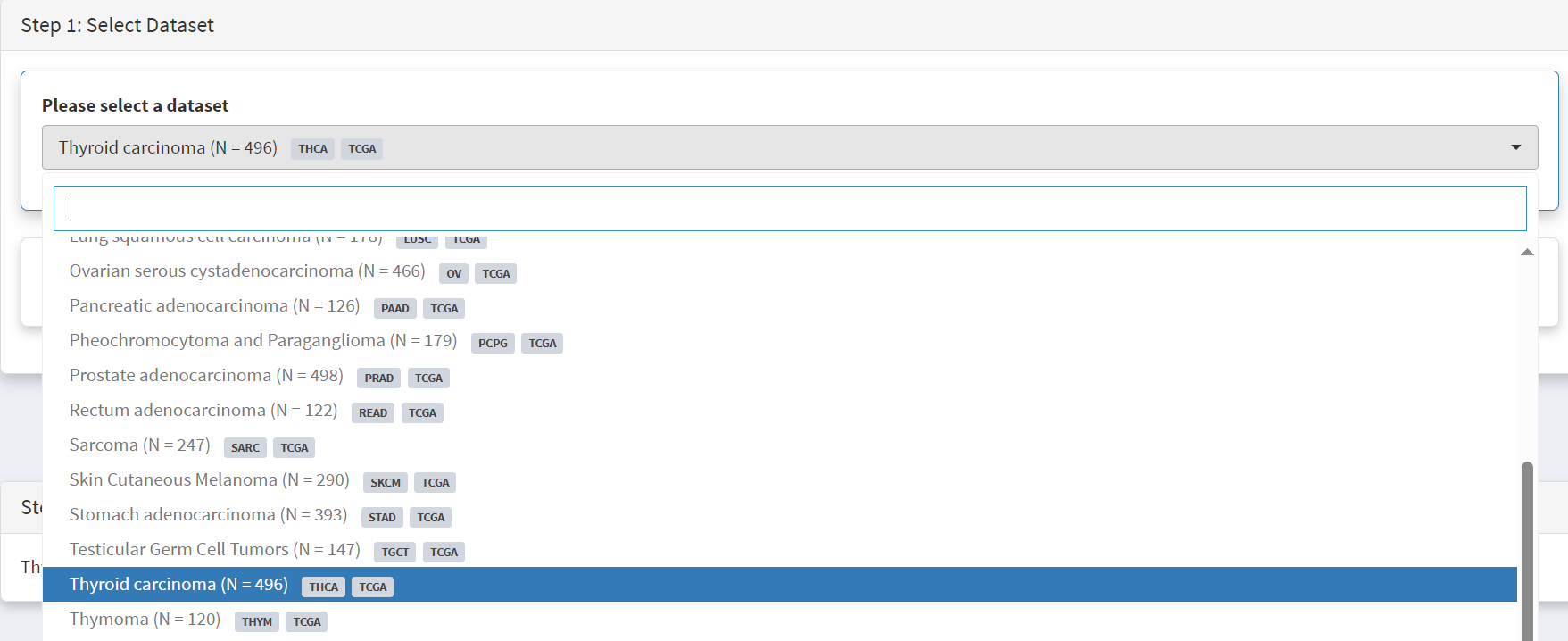
For this study the first step from the CRUX homepage is to select and load the thyroid carcinoma dataset. This is available from ‘Available Data’ module, accessible via either the data menu on the sidebar or the ‘Explore Public Datasets’ button in the ‘Getting Started’ homepage panel. The thyroid carcinoma dataset (THCA) dataset is brought up by typing ‘thyroid’ in the name field [screenshot 1] or THCA into the abbreviation field.
Screenshot 1
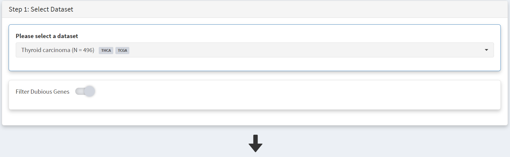
Clicking on the dataset ‘Thyroid_carcinoma’ button opens the cohort summary page; the Filter Dubious Genes toggle on Step 1 panel [screenshot 2] is enabled.
Screenshot 2
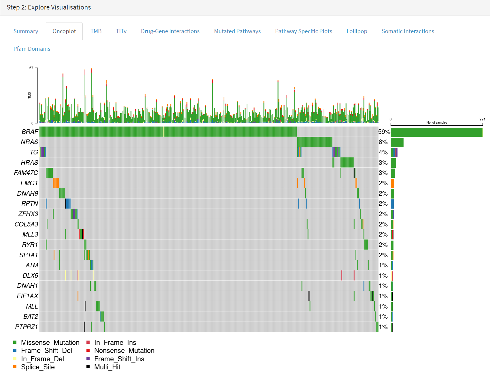
Below this in the Step 2 panel there are the Explore Visualisation tabs [screenshot 3]. Here we use the Oncoplot tab to examine the genes with mutations occurring in the largest number of samples. The standout gene is BRAF, although NRAS, HRAS, FAM47C and TG are also notable. The NRAS and HRAS are known oncogenes, FAM47C is a poorly understood but widely expressed gene, while TG is a significant THCA marker (encoding the thyroglobulin protein produced by thyroid tissue) which may not be oncogenic.
Screenshot 3
Use of OncoDriveCLUSTL tool.
OncoDriveCLUSTL is an external platform for gene driver analysis. This is accessed using the External Tools button on the CRUX sidebar. On the page that opens, the first step is to select the THCA dataset for export at the Step 1 panel, as shown in screenshot 4.
Screenshot 4
Then Filter Dubious Genes is selected [screenshot 5].
Screenshot 5
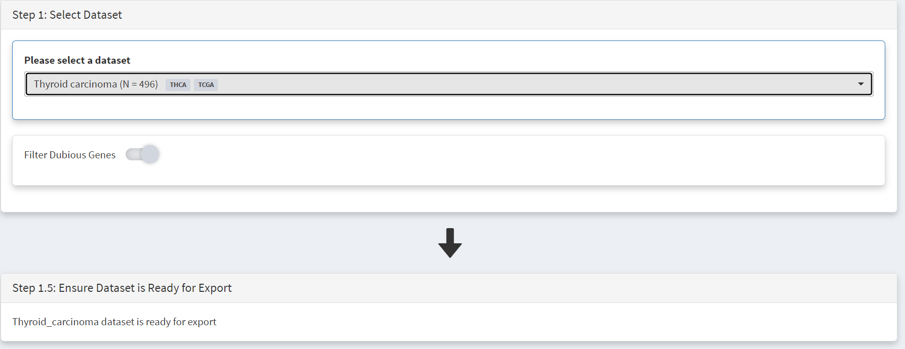
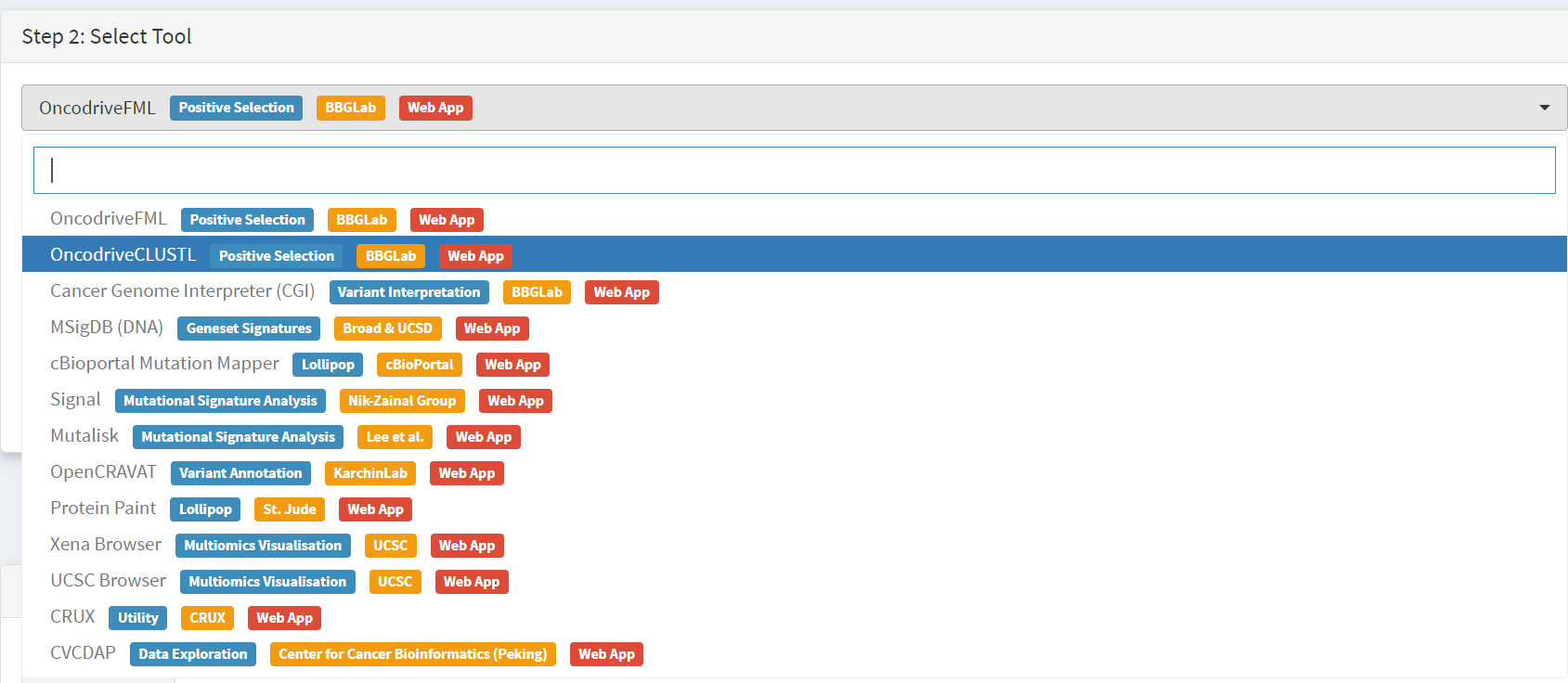
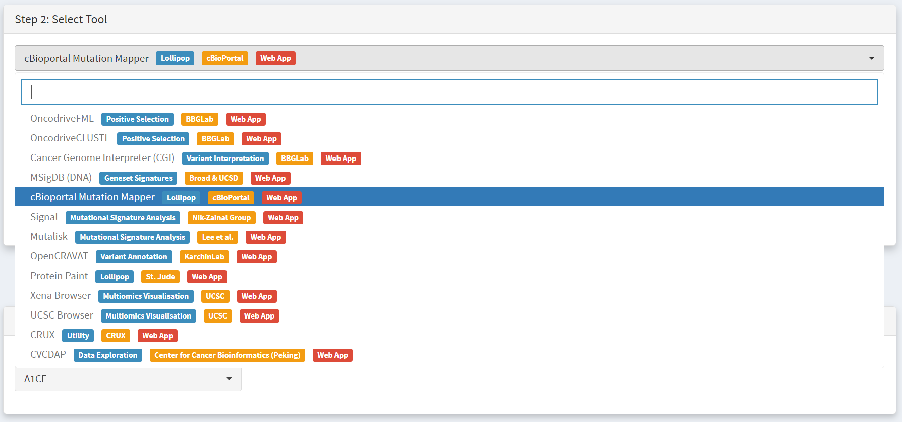
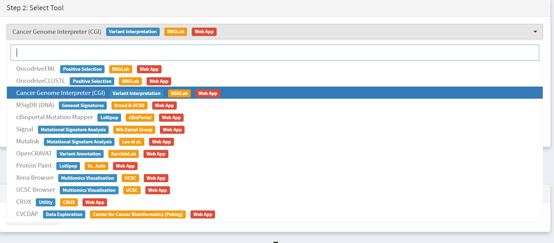
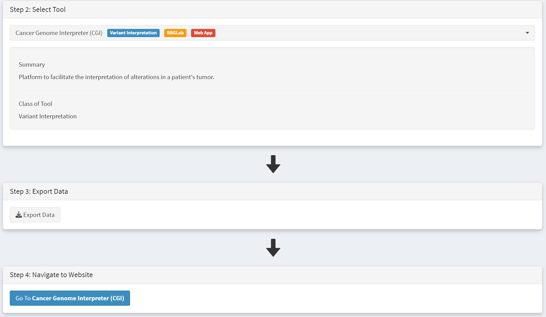
Below this is the Step 1.5 panel, where CRUX should indicate the THCA dataset is ready for export. In the step 2 panel there is the Select Tool tab. By default the first tool (OncodriveFML) is selected, but when clicked a drop-down menu appears listing all options, allowing OncoDriveCLUSTL to be selected [screenshot 6].
Screenshot 6
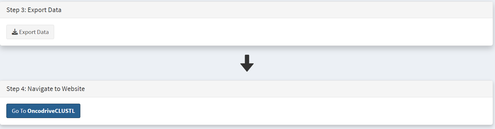
Moving to the Step 3 panel [screenshot 7], clicking on the Export Data button will download the formatted THCA dataset to the user computer, ready to upload to the OncoDriveCLUSTL platform. On the Step 4 panel, clicking on the blue button opens a new browser window for OncoDrivCLUSTL, at http://bbglab.irbbarcelona.org/oncodriveclustl/analysis :
Screenshot 7
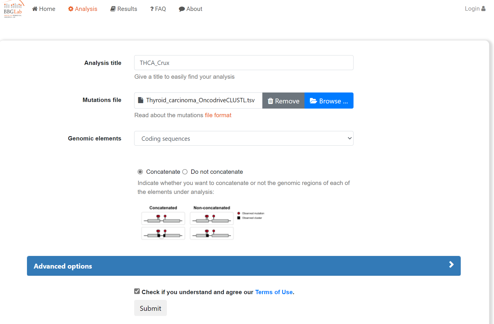
On the Step 5 panel (not shown) there are instructions and information on the tool. To use OncoDriveCLUSTL a BBGlab account is required (this is free and quick to set up). Once you log in, to run OncodriveClustl simply give the analysis run a name then upload the THCA file prepared by CRUX [screenshot 8].
Screenshot 8
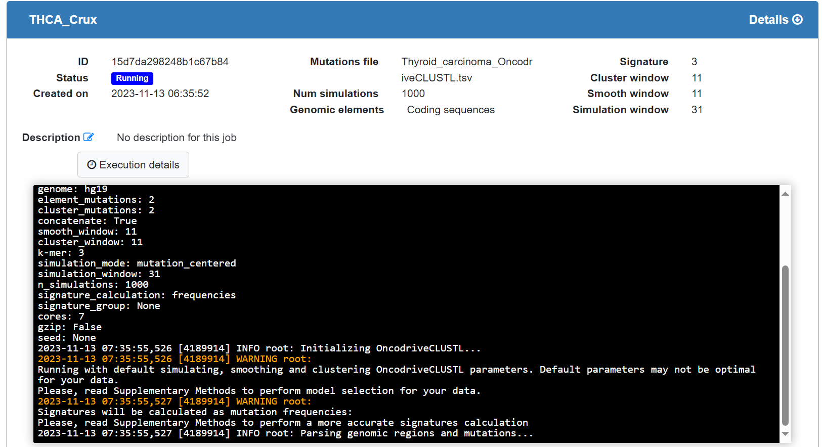
After checking the terms of use button and pressing submit a process progress window opens; screenshot 9 was taken shortly after starting a data processing run.
Screenshot 9
The data processing may take some time, over 15 minutes for this dataset. The window will show the status indicator as ‘Finished’, and a plot appears [screenshot 10] showing genes whose mutation appears to be positively selected (putative drivers) with observed versus expected p-values.
Screenshot 10
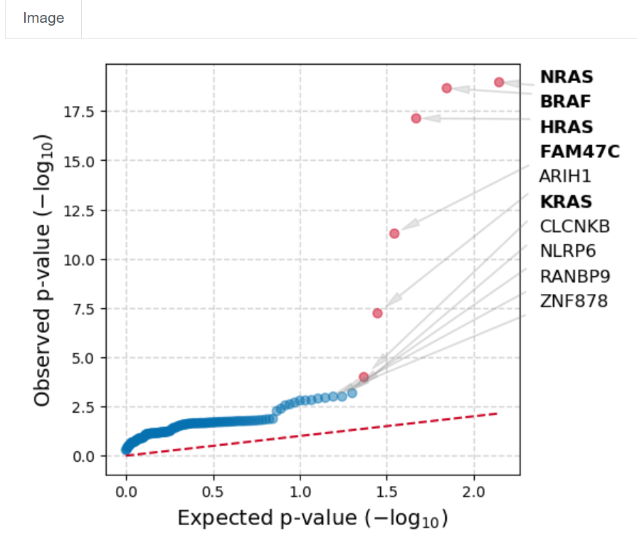
This indicates that BRAF, NRAS, HRAS and FAM47C mutations (seen in Oncoplot) are highly selected for standout candidates to be examined. Note that TG is not seen.
In the next part of the study we examine BRAF mutations.
Use of cBioPortal mutation mapper tool
As above the External tools tab is selected from the CRUX home page, the THCA data is selected and cBioPortal mutation mapper is chosen in the Step2 panel as the tool we want to export data for [screenshot 11].
Screenshot 11
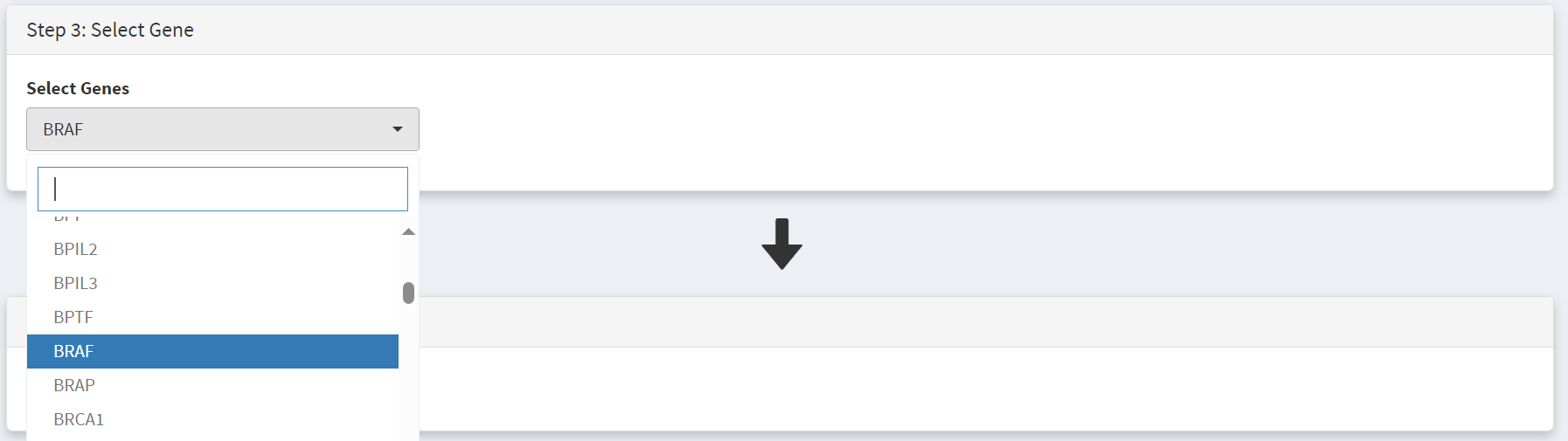
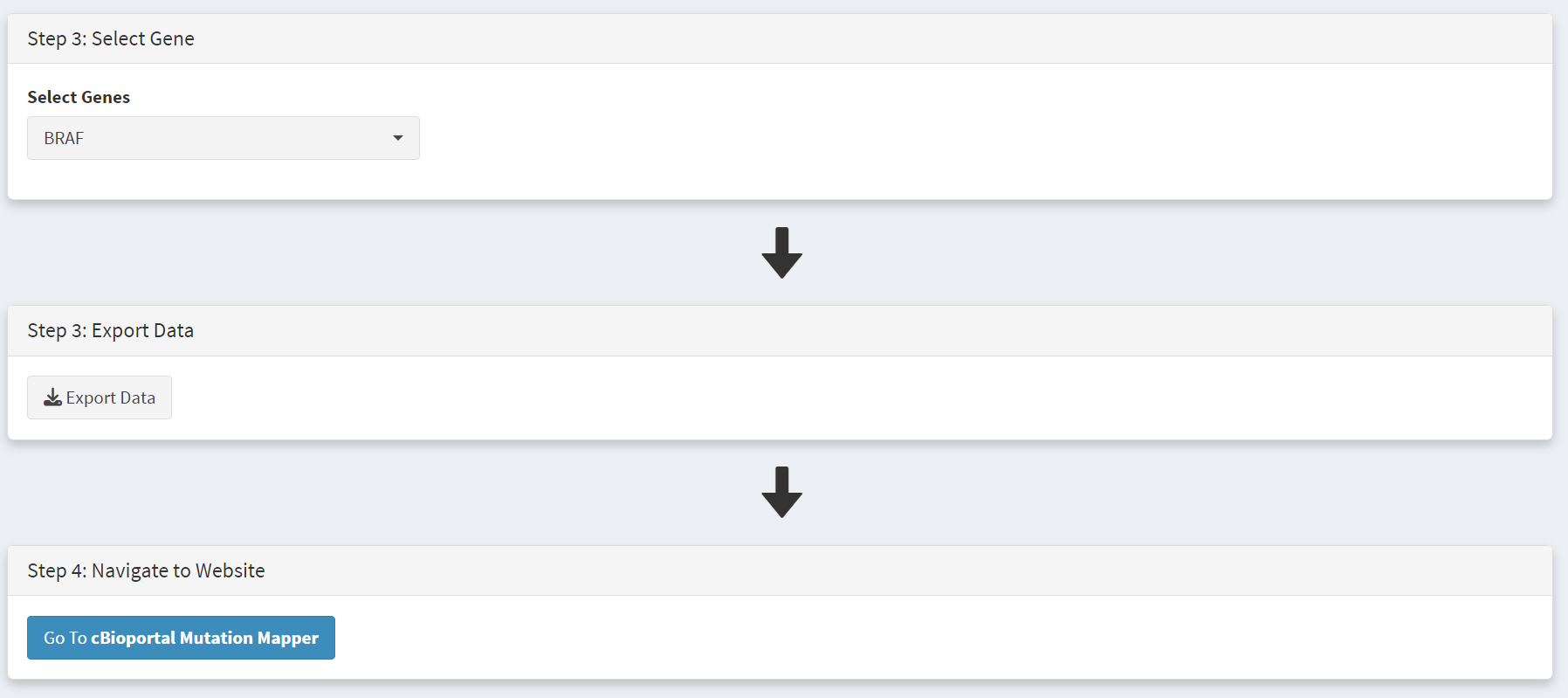
We then need to select the gene, BRAF, in the step 3 panel [screenshot 12].
Screenshot 12
We then use the ‘Export Data’ button to download the data as we did for oncodriveClustl, and use the ‘Go to cBioportal Mutation Mapper’ button on the Step 4 panel to navigate to the tool at https://www.cbioportal.org/mutation_mapper.
Screenshot 13
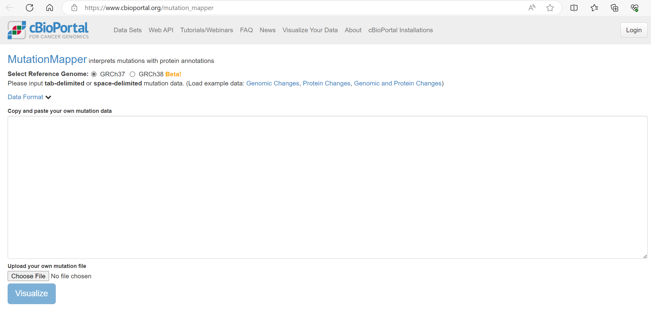
The cBioportal Mutation Mapper window is shown in screenshot 14.
Note for this TCGA dataset the reference genome GRCH37 selected.
The mutations file is uploaded using the ‘Choose File’ button, then we click Visualise [screenshot 15].
Screenshot 14
Screenshot 15

A plot is returned, shown in screenshot 16.
Screenshot 16
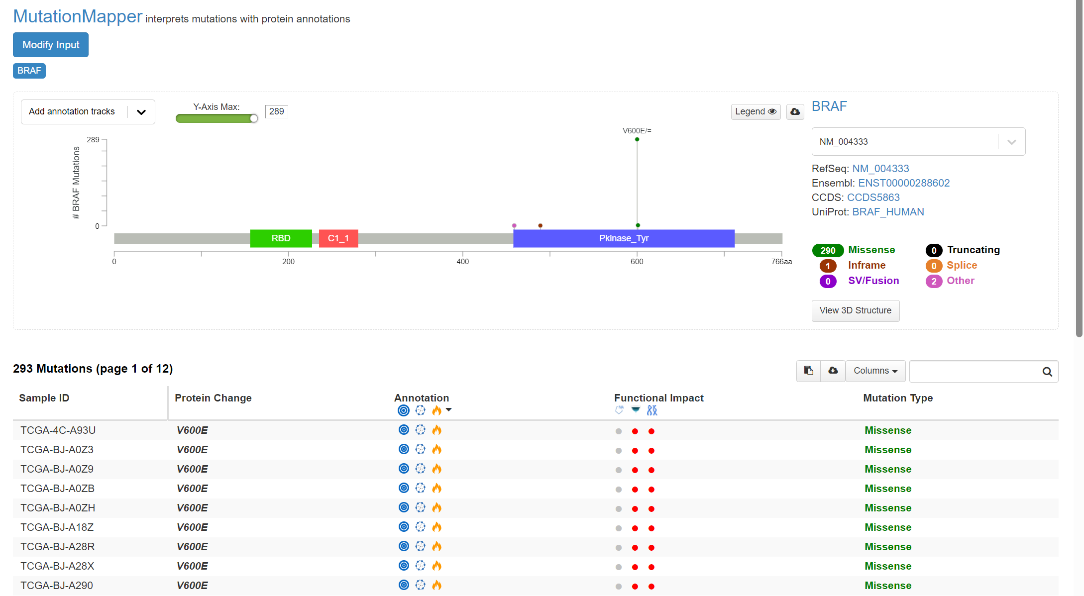
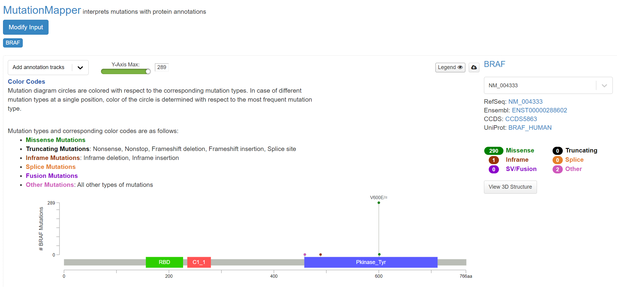
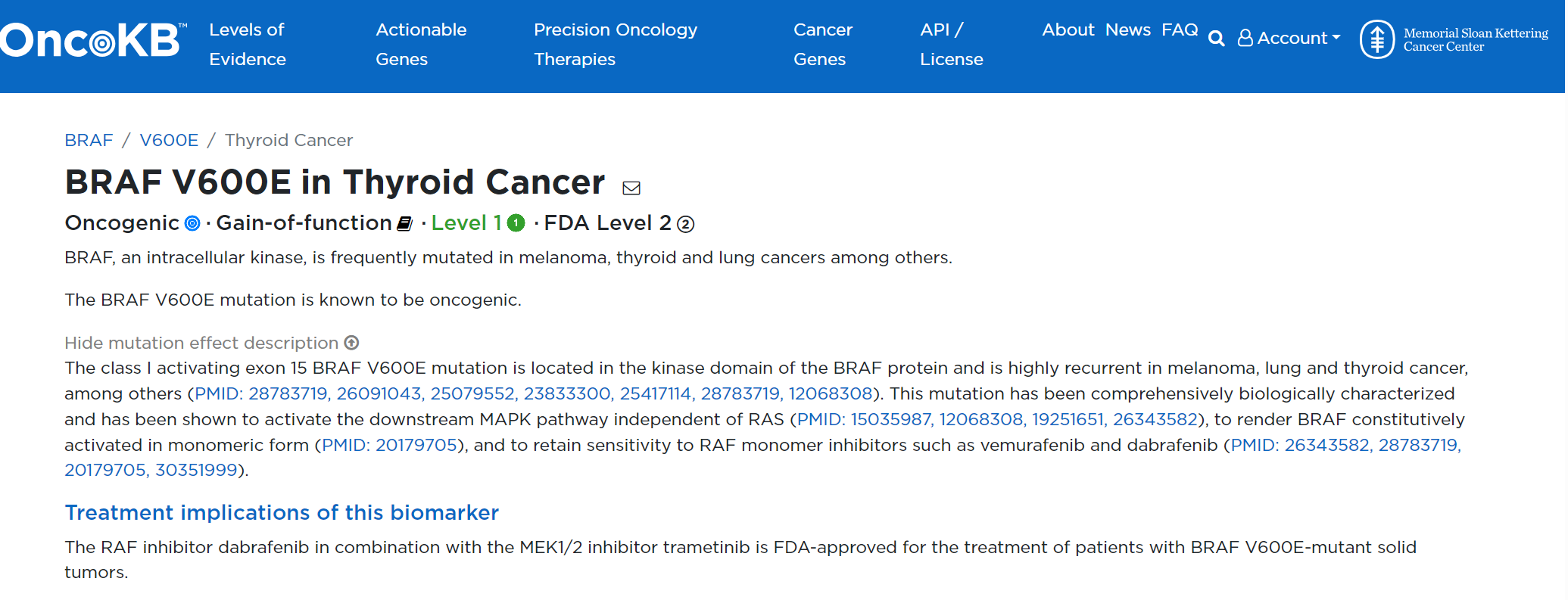
This indicates the gene domains and the presence of mutations, as well as the mutation types and their annotations from OncoKB and others. A plot with the mutation type legend is shown in screenshot 17.
Screenshot 17
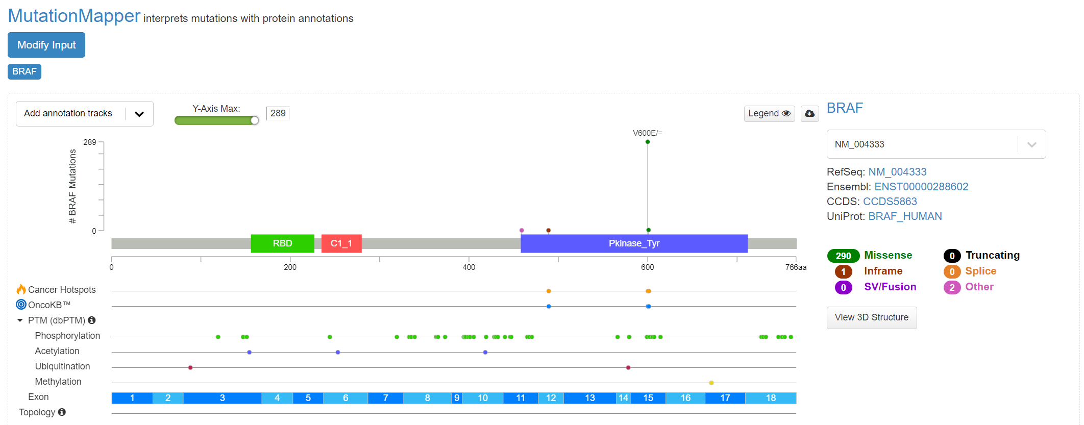
Further details of cohort mutations can be added [screenshot 18], using the ‘Add annotation tracks’ button, seen in screenshot 18. A 3D protein structure graphic showing the affected domain can also be obtained (not shown).
Screenshot 18
Use of Cancer Genome Interpreter (CGI) tool
After navigating to the External tools on the home page, the CGI tool Is selected [screenshot 19].
Screenshot 19
The THCA dataset is selected and exported [screenshot 20] as described previously.
Screenshot 20
Clicking on the navigation button in the Step 4 panel opens a new browser window for the CGI portal [screenshot 21] at https://www.cancergenomeinterpreter.org/analysis; an account (easily obtained and free) is needed for login. If not logged in the tool can work, but it is likely that there will be a pink box at the bottom indicating ‘you have exceeded the maximum number of jobs’. Log in will make the user’s previous analyses from the previous 6 months available.
The ANALYSIS tab should be open for the next step.
Screenshot 21

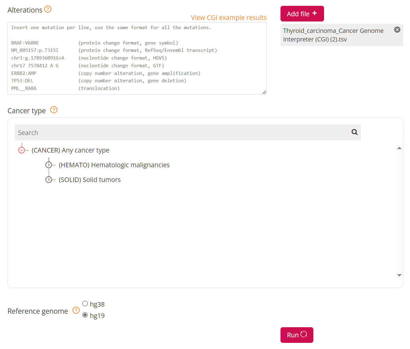
Clicking on the Add File button will allow upload of the CRUX-formatted dataset. For this THCA dataset note the reference genome is hg19; this is selected and Run button pressed [screenshot 22].
Screenshot 22
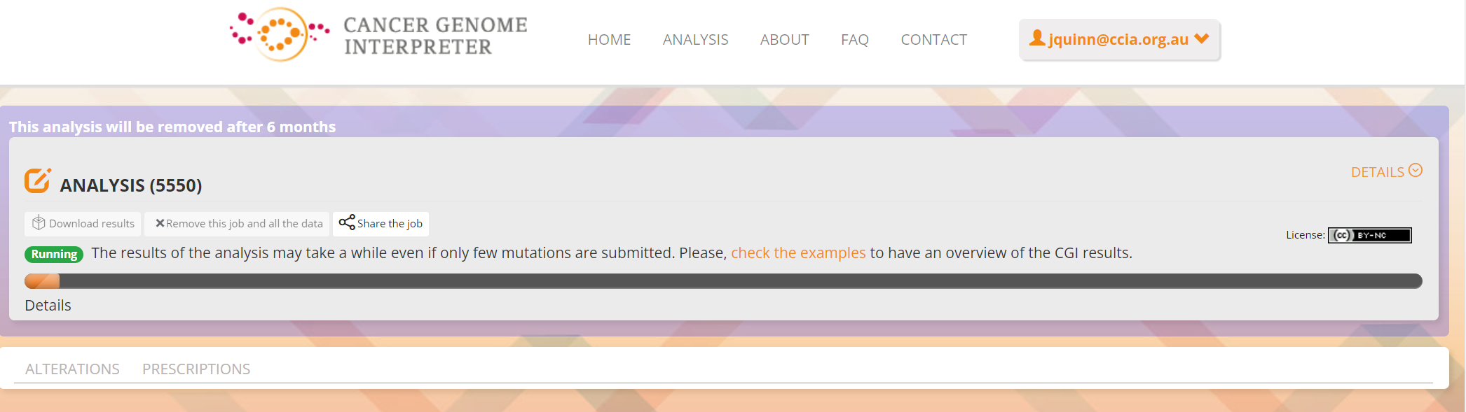
The job will start running (this will take some minutes) and the progress bar will resemble screenshot 23.
Screenshot 23
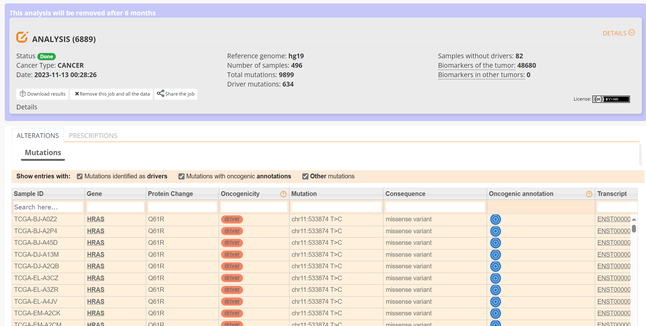
Processed data can be downloaded from the site. There will be a configurable table of patient samples, as seen in screenshot 24 for the initial view of the ALTERATIONS tab. Note the ‘drivers’ indicated under Oncogenicity.
Screenshot 24
This table can be explored in various ways: gene of interest or sample of interest can be selected, driver information obtained (clicking on the driver buttons bring up the CGI boostDM tool) and annotation from OncoKB, clinvar and CGI databases. These are selected by clicking on the symbols in the Oncogenic annotation column. One example for BRAF is shown in screenshot 25, which indicates the mutation is gain of function.
Screenshot 25
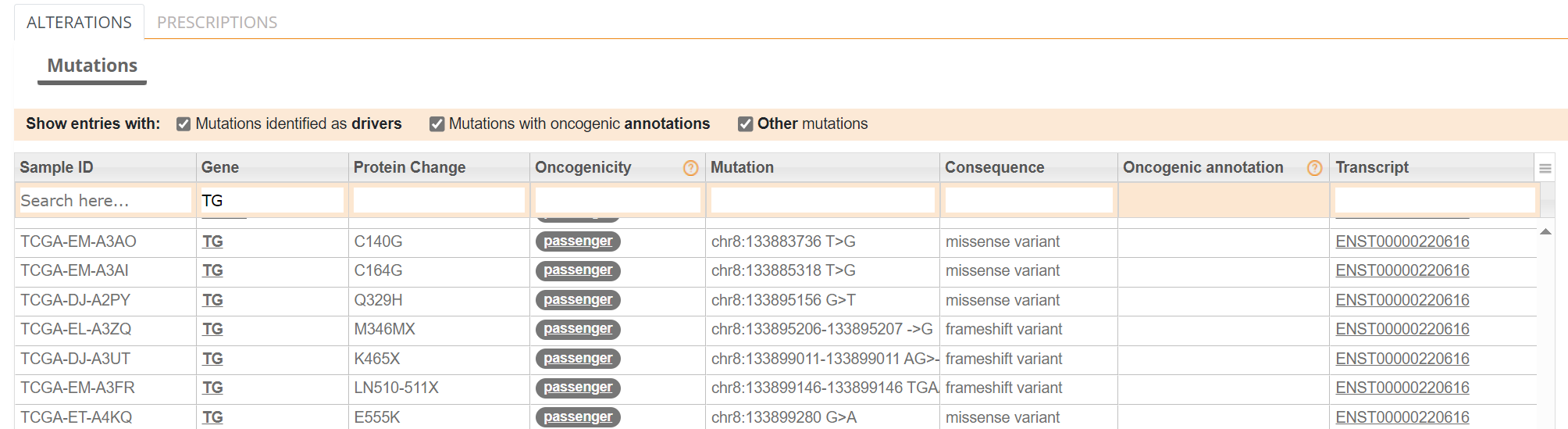
Examining TG gene mutations on the ALTERATIONS table, these are confirmed as passenger mutations [screenshot 26]:
Screenshot 26
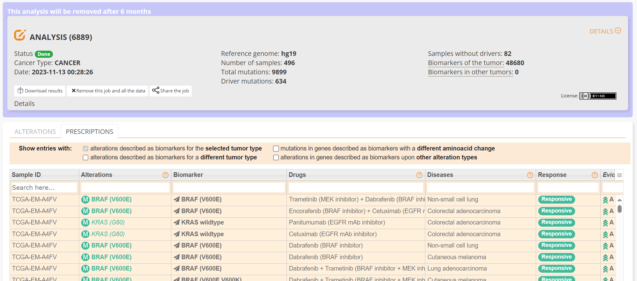
The PRESCRIPTIONS tab results are shown in screenshot 27, giving information on the drugs used in patient care and whether the mutations make the cancer resistant or still responsive.
Screenshot 27
Short study 4: Mutational Signatures
Mutation signature analysis of cohort data.
Dataset: We created a new dataset in CRUX by importing data from a previously published study of 30 lung tumours sequenced with deep multi-region whole genome sequencing (WGS). These data are from the Leong et al 2019 (PMID: 30348992). Raw data is available from European Nucleotide Archive (https://www.ebi.ac.uk/ena) accession number PRJEB28616. The patients included current, former, and non-smokers, and the tumour biopsies were from paired primary and metastatic tumour biopsies. The data was originally in VCF file format, which we annotated using a command line vcf2maf tool available at https://github.com/mskcc/vcf2maf to create the MAF files employed here. Further clinical annotation used data (CSV filetype) on patient smoking status.
Note
There are now more accessible ways to convert VCF files to MAFs if you are not comfortable working on the commandline
In this study we examine somatic variant signatures in lung cancer data. These signatures are patterns of single nucleotide mutations which can provide mutagenesis mechanisms and other information regarding tumour development; the signatures used are COSMIC V3. Analysis employed two external tools, Mutalisk (http://mutalisk.org/analyze.php) and Signal (https://www.signaldb.org/). For this work MAF files must first be imported to CRUX, alongside clinical data (smoking status of participants).
To get started we navigate to the Import Data module (available under the Data menu on the CRUX sidebar) [screenshot 1]. After selecting MAF filetype in the Step 1 panel, the relevant MAF file was chosen was located using the Browse button in the Step 2 panel and imported.
Screenshot 1
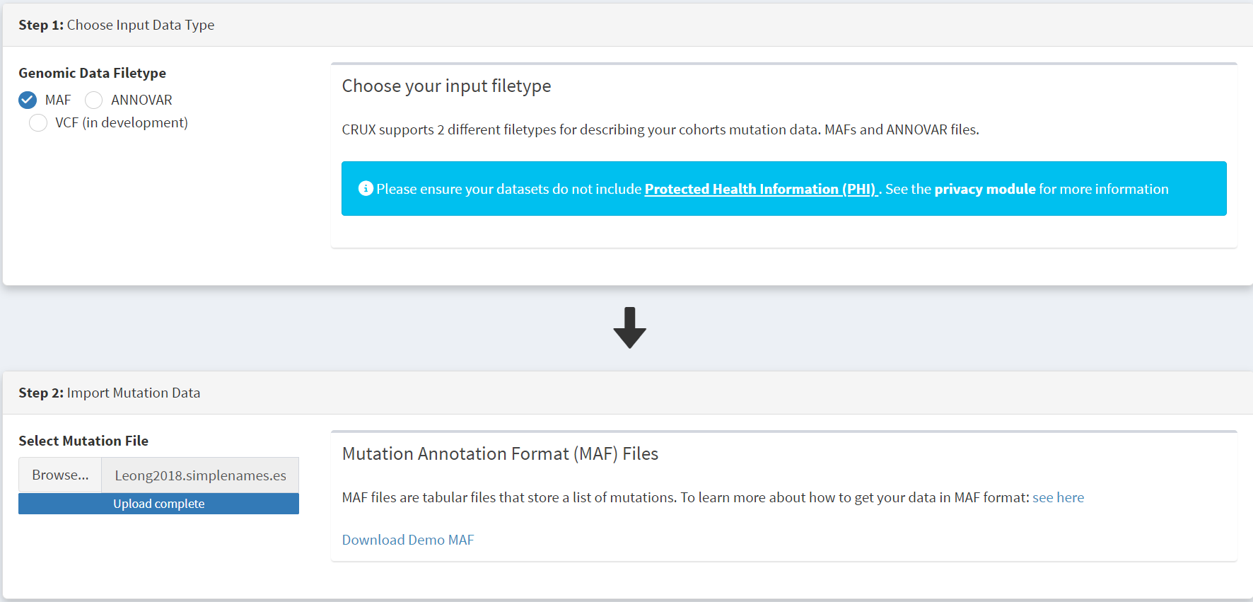
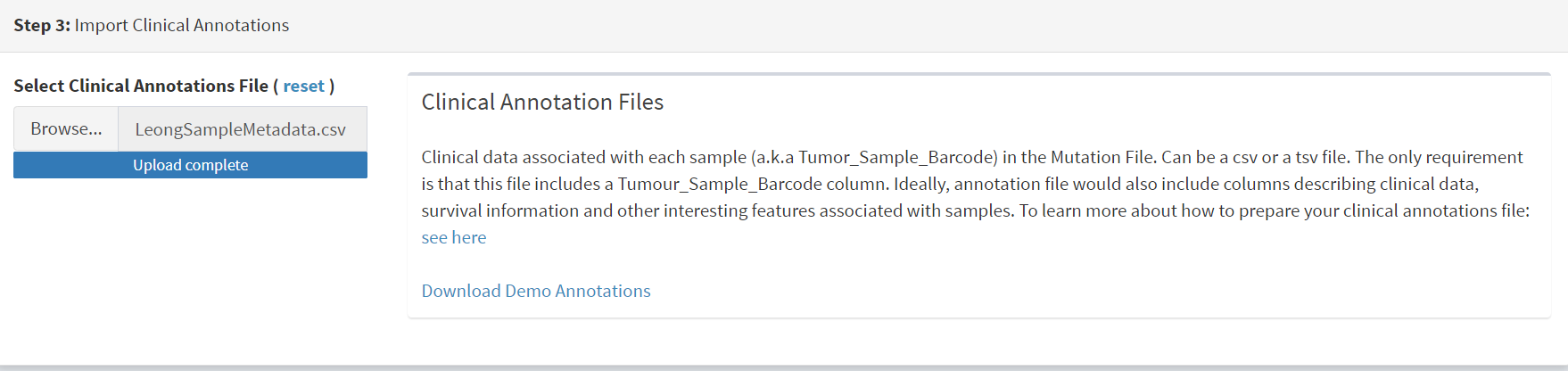
The additional clinical annotations file was similarly located, selected and uploaded from the STEP 2 panel [screenshot 2].
Screenshot 2
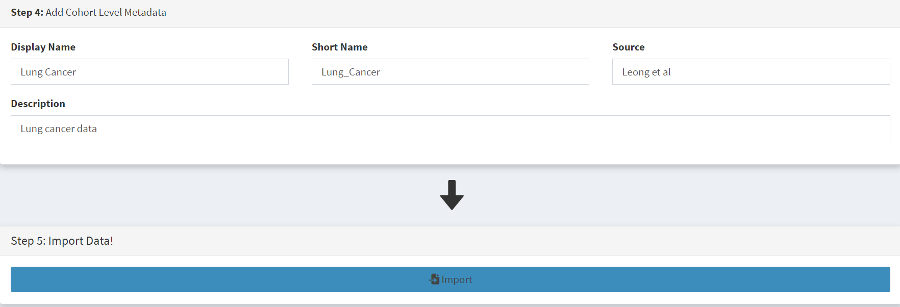
In the Step 4 panel the files were then given the name (‘Lung Cancer’) that they will carry when loaded in CRUX. The Import button (blue) was then pressed [screenshot 3]
Screenshot 3
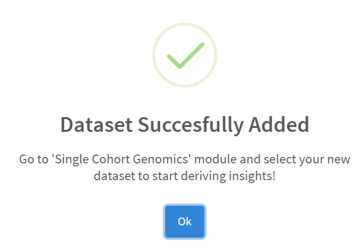
Import to CRUX was confirmed after 20 second delay [screenshot 4].
Screenshot 4
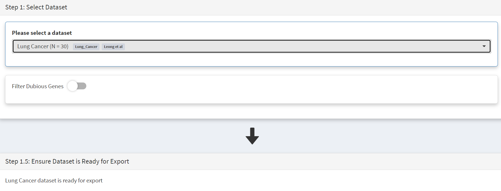
Selecting the External Tools (CRUX sidebar) opens a page where the dataset is chosen [screenshot 5]. Note that the Dubious Genes filter is not selected as the passenger mutations in these genes may still be useful for in the signature analyses.
Screenshot 5
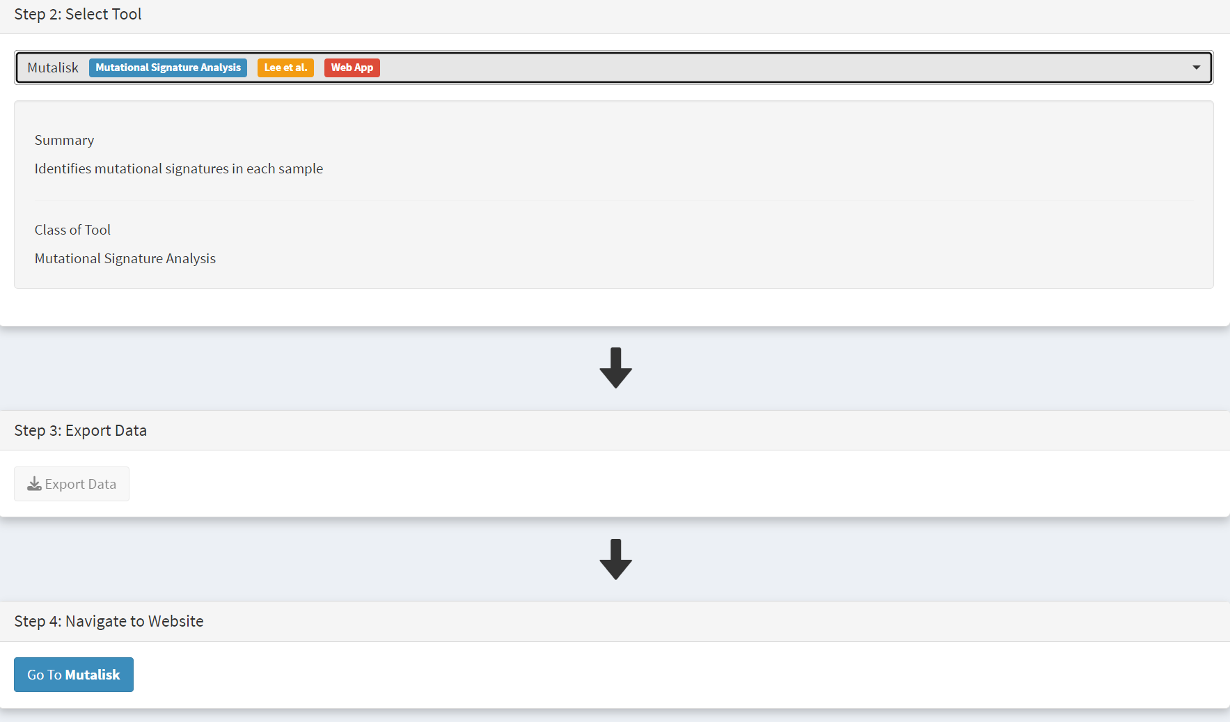
In the External Tools Step 2 panel ‘Mutalisk’ is selected, and the data exported at Step 3; this arrives in the computer download folder as a zipped folder called ‘Lung Cancer_Mutalisk’, the dataset name in CRUX. This contains VCF data files for all the samples, and it is best to unzip this folder before proceeding further. These individual files will be uploaded to Mutalisk as described below.
Note that in the Step 5 panel there is information about using Mutalisk:
Instructions
Unzip exported file
Click ‘Upload Files’ and select all samples you want to run signature analysis on
Select reference build (Human GRCh37 if using pre-packaged TCGA/PCAWG datasets)
Select the relevant Disease Type (mutalisk will automatically choose relevant signatures to screen in sample). An alternate unbiased approach is to screen against the full set of PCAWG (V3) signatures. To do this expand the PCAWG tab and ‘select all’ signatures. You do not need to specify a disease.
Run analysis
Next press the Go to Mutalisk button selected in Step 4 panel [screenshot 6].
Screenshot 6
CRUX then opens a browser window running Mutalisk [screenshot 7].
Screenshot 7
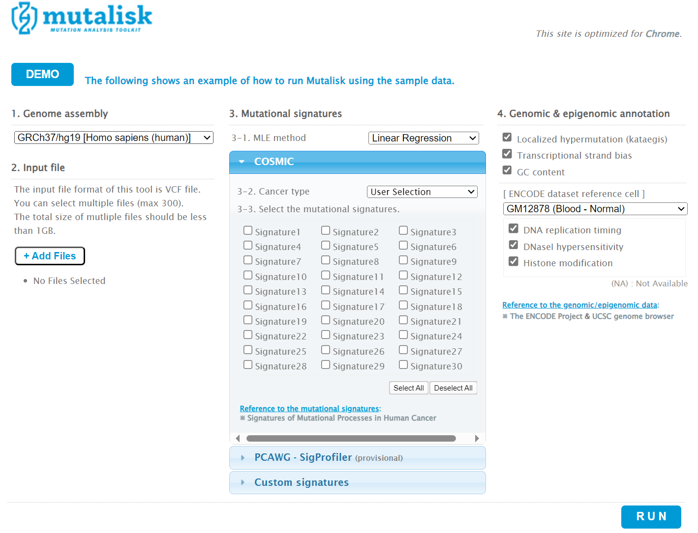
However, the ‘COSMIC’ signatures are not the most up to date. To select the correct type of COSMIC V3 signatures it is necessary to select the PCAWG – Sig profiler option below it. Then the signature types to be examined are designated using the Select all button [screenshot 8].
Screenshot 8
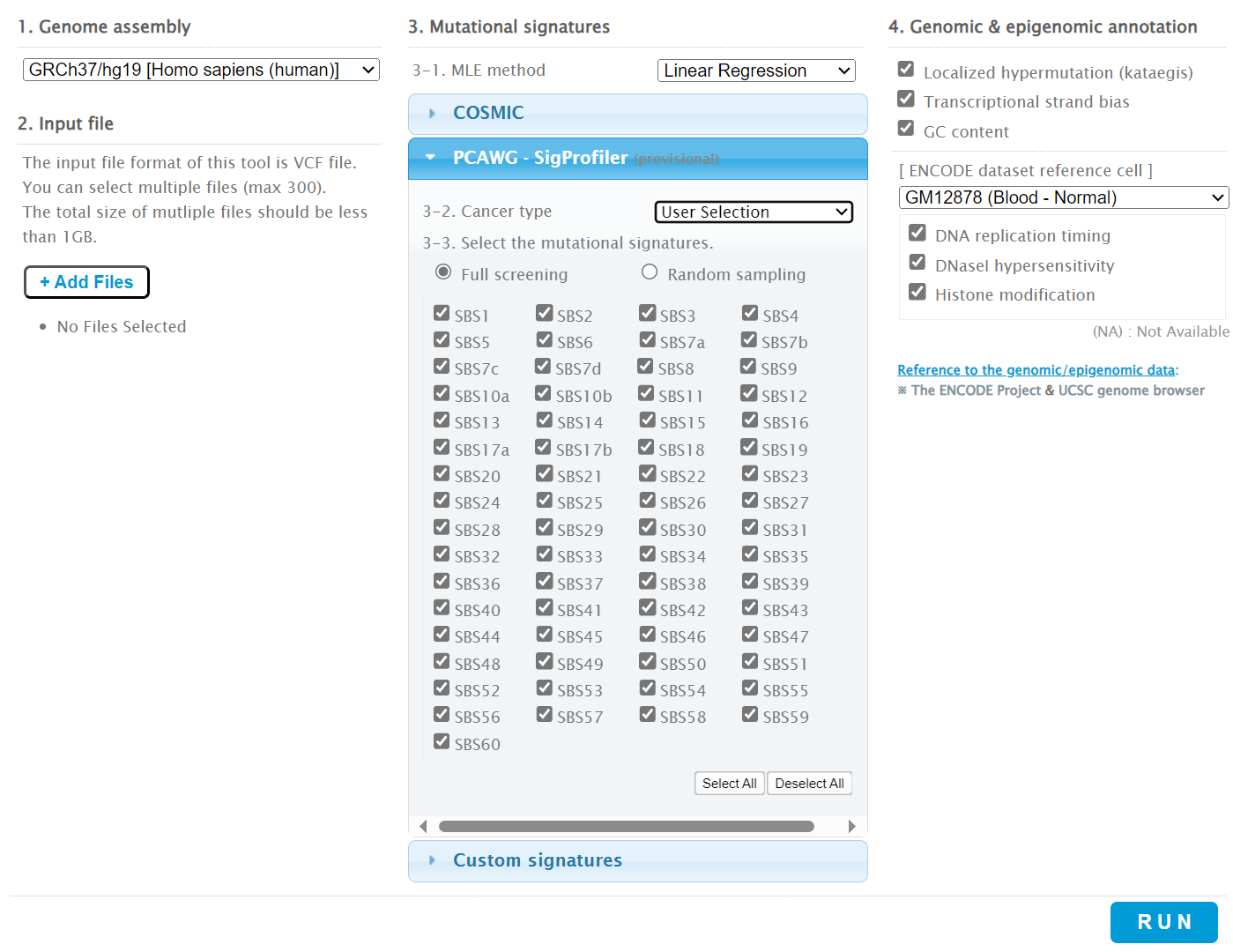
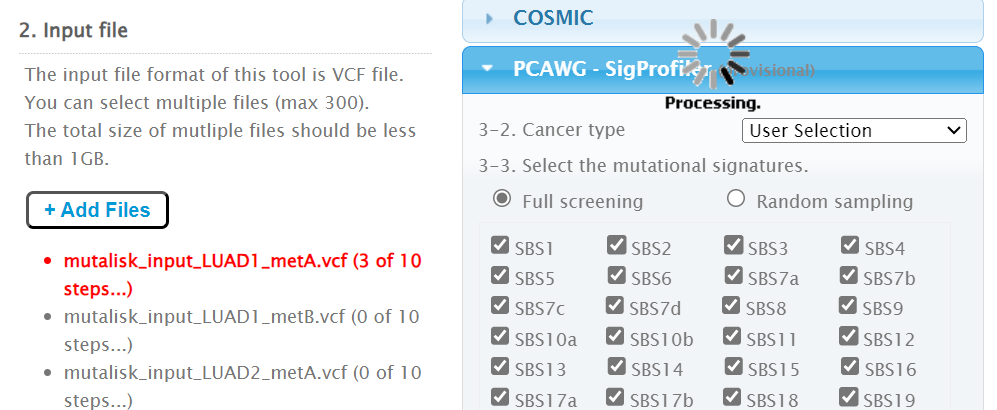
Then the +Add Files option is pressed, the files exported from CRUX are chosen (unzipped) and the files are processed [screenshot 9]. The RUN button is then pressed and the analysis proceeds as indicated. Note that this processing is slow and can take several hours for 30 samples. The initial stage of processing is shown in screenshot 9. Mutalisk gives a process number so the user can exit and return to see progress later.
Screenshot 9
Mutalisk then outputs a number of analyses for each dataset input. Examples for LUAD1 are shown in screenshots 10 to 13. For example, screenshots 10 and 11 show kataegis analysis output for LUAD1 and LUAD7, respectively, showing a predominance of C>A mutations in the latter but not the former.
Screenshot 10
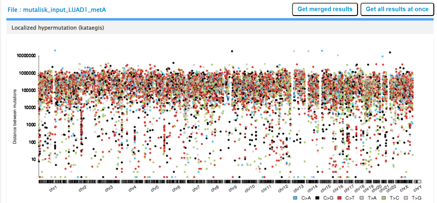
Screenshot 11
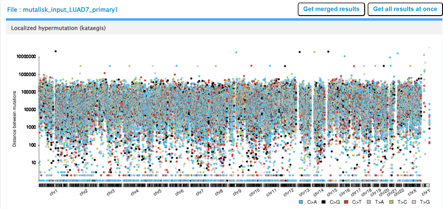
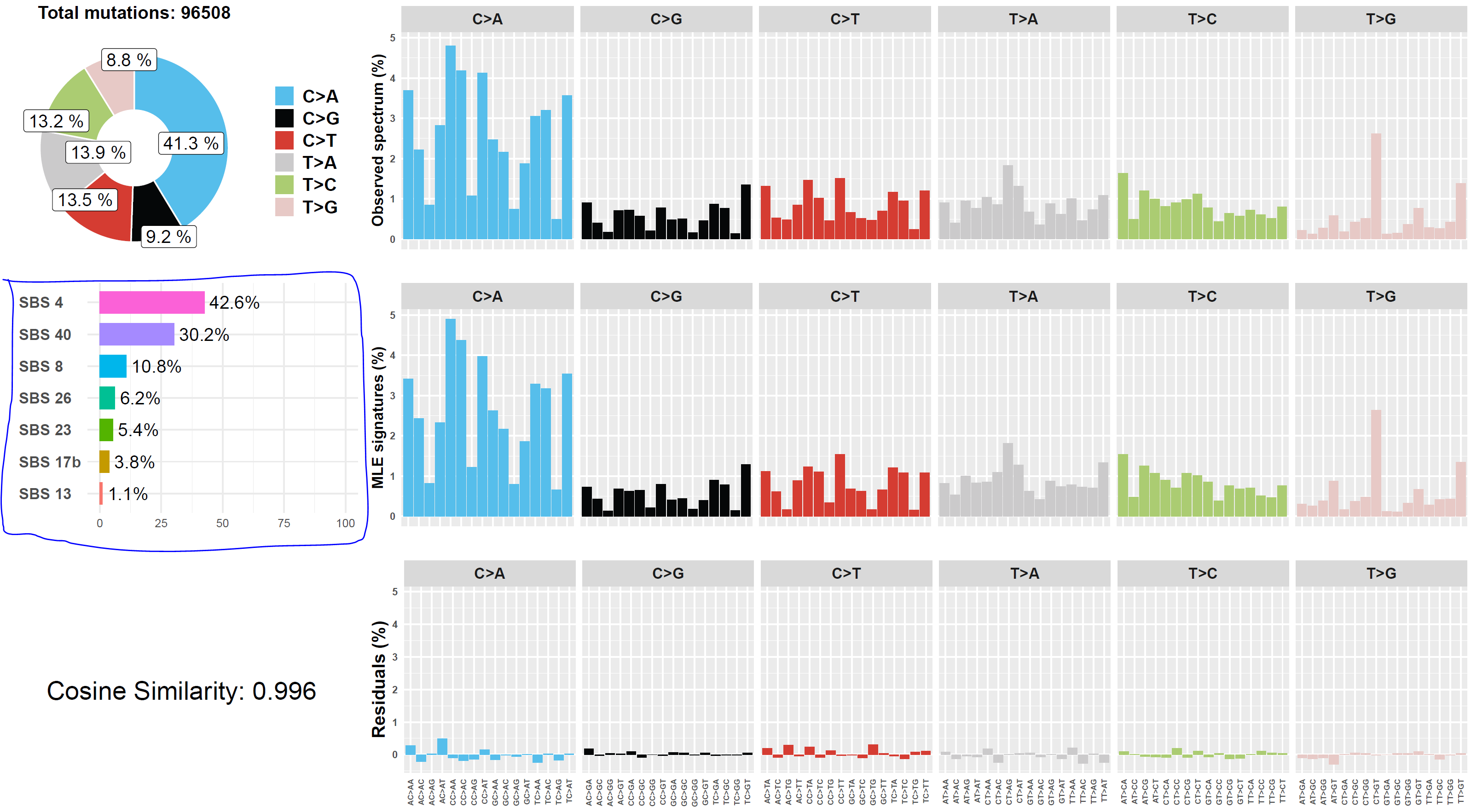
Screenshot 12 shows the Mutalisk signature output from sample LUAD7_primary1, a primary lung tumour showing a typical smokers profile with high SBS4. Highlighted (blue line) is the signature plot presented in El-Kamand et al Figure 5C (recoloured for clarity).
Screenshot 12
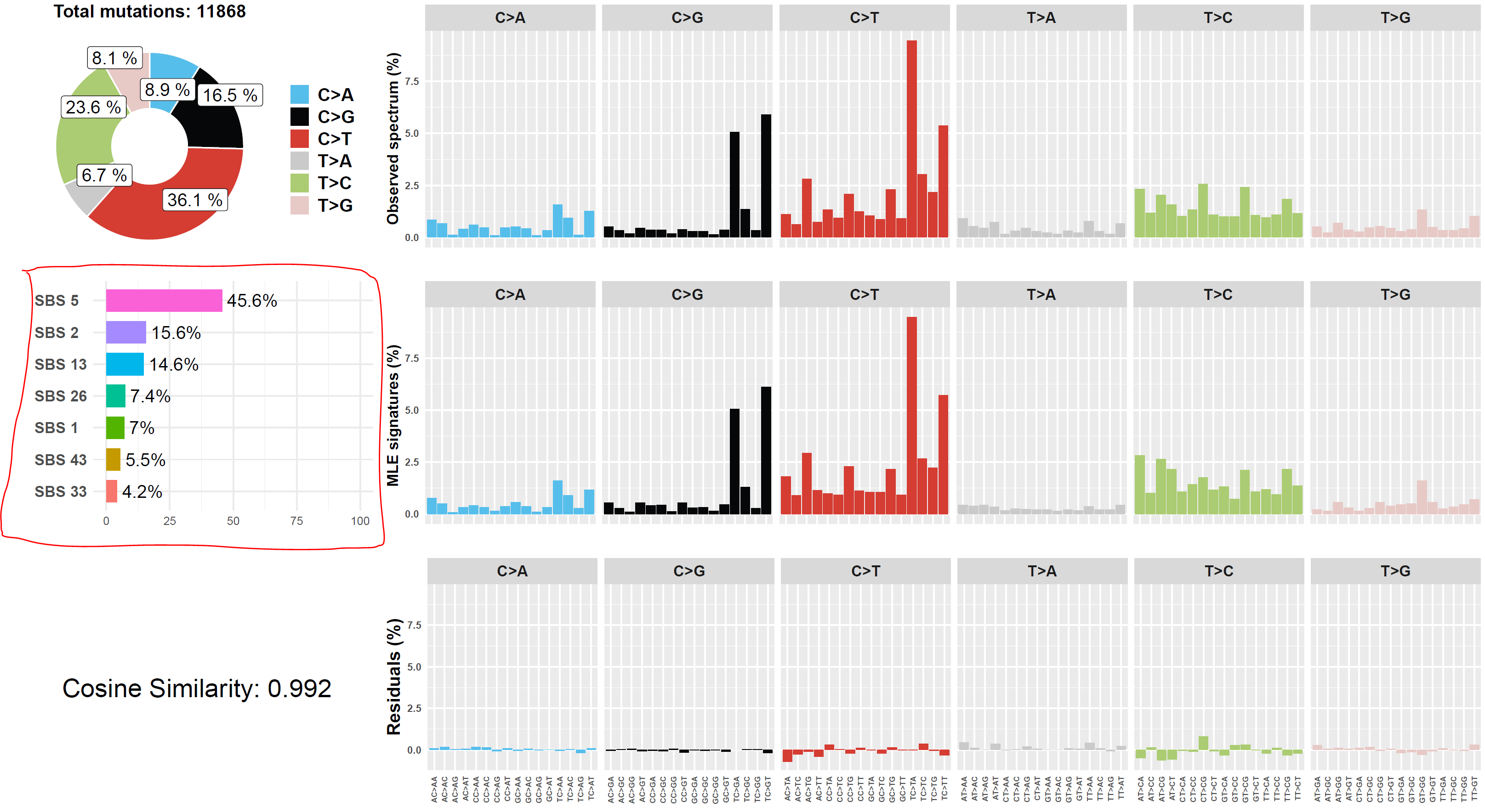
Screenshot 13 shows the Mutalisk signature output from sample LUAD1_metA, a lung tumour metastasis showing a non-typical smokers profile no detectable SBS4. Signature plot is highlighted (blue line) in El-Kamand et al Figure 5C (recoloured for clarity).
Screenshot 13
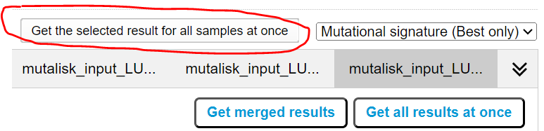
However, for cohort wide analysis we need to load the Mutalisk data back into CRUX. At the top of the Mutalisk page the ‘Get the selected result for all samples at once’ button is pressed [screenshot 14, red line highlight].
Ensure the results mutalisk is set to download only the best model for each sample by selecting ‘Mutational Sigature (Best Only)’ in the dropdown to the right of the ‘Get the selected result for all samples at once’ button as pictured in [screenshot 14]
Screenshot 14
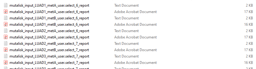
This downloads a zip file with a filename ending in ‘.all.samples.zip’. The next step uses these files downloaded from Mutalisk, which are first unzipped; example mutalisk files from a containing folder are shown in screenshot 15.
Screenshot 15
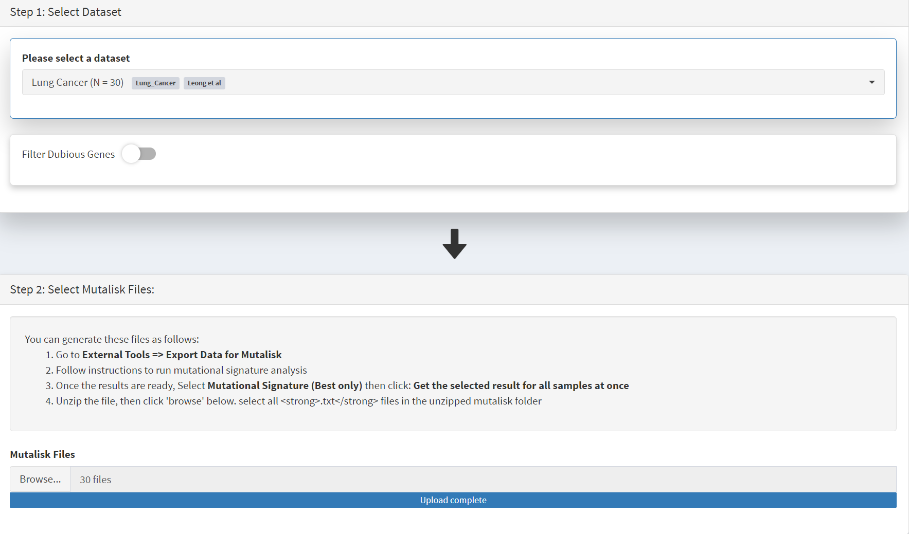
When the Mutalisk files are ready, the Mutational Signatures tab (under the Single Cohort Genomics menu located on the CRUX sidebar) is then selected to open a new page of panels [screenshot 16]. On the first (Step 1) panel the Lung Cancer data is selected using the ‘Please select a dataset’ field. We leave Filter Dubious Genes of since it will have no effect on this module. Then we note that the Step 2 panel includes instructions on how to prepare the mutalisk files - these have already been followed by this point. The next actionis to press the Browse button, and navigate to where the unipped Mutalisk files are located and select all your mutalisk reports (navigate to folder and hit [ctrl + A] or [command + A]). Those files are selected and opened by CRUX, which may take a minute. When finished the blue ‘Upload Complete’ bar should appear below.
Screenshot 16
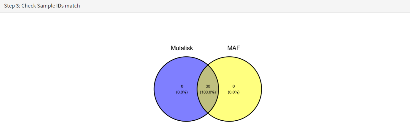
The next panels should then be visible. Step 3 panel shows a Venn diagram indicating that the MAF and Mutalisk data match up [screenshot 17].
Screenshot 17
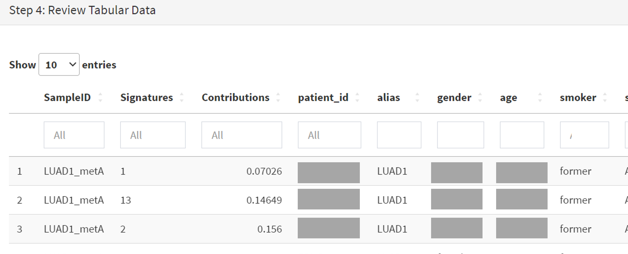
The Step 4 panel (Review Tabular Data) contains the data table, including the signature variants and their contributions for each sample; part of the table is shown on screenshot 18. This data can be subsetted and searched but is more easily comprehended in the next Step.
Screenshot 18
The Step 5 panel [screenshot 19] shows the visualisation of the signature contributions (X-axis) for each tissue sample. Note that chart colours in the El-Kamand et al manuscript have been adjusted for clarity.
Screenshot 19
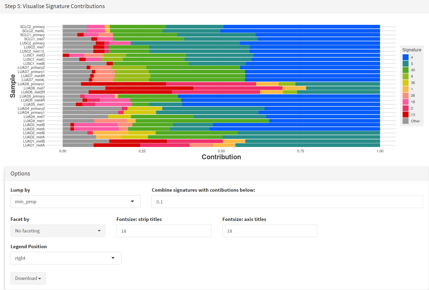
Note
The options panel below the plot includes a ‘facet by’ menu, which lets us group samples by their smoking status, and helps produce the effect observed in the El-Kamand et al manuscript.
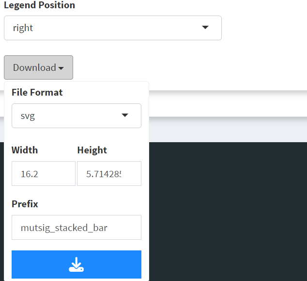
Pressing the Download button at the bottom brings up the download options shown in screenshot 20.
Screenshot 20
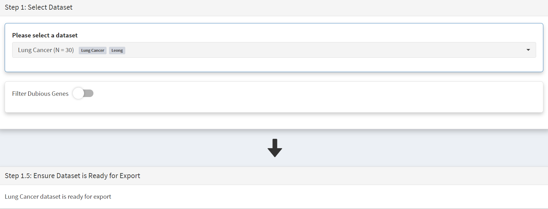
Next further signature analysis can be performed using the external Signal tool with the Lung cancer data loaded into CRUX as above.
As for Mutalisk above, we first navigate to the External tool tab on the sidebar and open that page. In the Step 1 panel the Lung Cancer dataset is selected [screenshot 21]
Screenshot 21
On the Step 2 panel the Signal tool is selected [screenshot 22] and the data for export is downloaded using the Export Data button. Note again that the Filter Dubious genes is off, since for signature analysis we are not concerned with gene drivers but the general pattern of mutations present compared to those seen in other cancers.
Screenshot 22
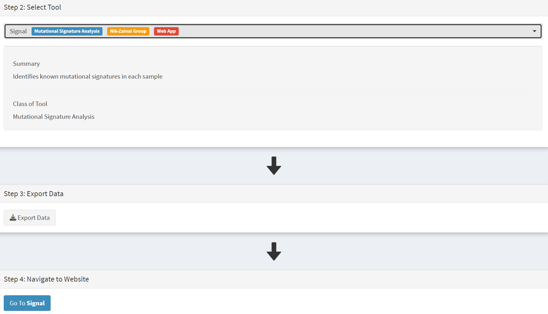
The filename zipped file provided is ‘Lung cancer_Signal.zip’. As described in the Step 5 panel, unzip the file (‘signal_input1.txt’) and navigate to the Signals portal (https://signal.mutationalsignatures.com/analyse2).
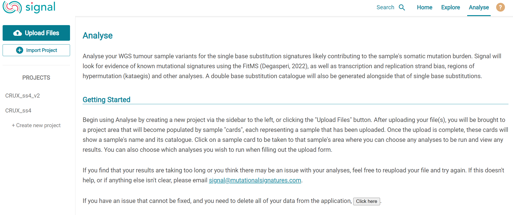
The blue Go to Signal button is press and Signal website opens in a new browser screen, as shown in screenshot 23.
Screenshot 23
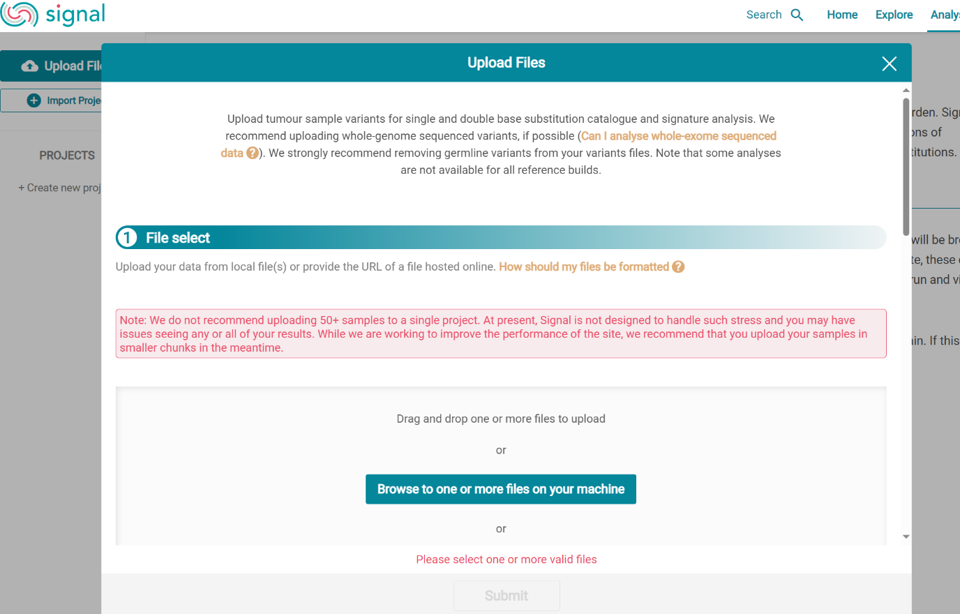
The upload data button is then pressed, which opens the upload file page [screenshot 24]. Here, the signal_input1.txt file from CRUX is uploaded according to instructions.
Screenshot 24
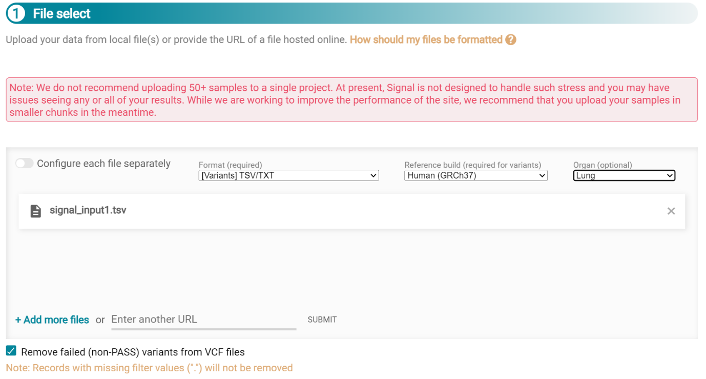
When the file finishes upload the file format must be selected as ‘[Variants]/TSV/TXT’ as seen in the screenshot 25. The reference genome build selected (here GRCh37) and the organ chosen, here LUNG.
Screenshot 25
When the analysis is done there are a number of panels that are used to access the analysis of individual lung cancer datasets; the first six shown in screenshot 26.
Screenshot 26
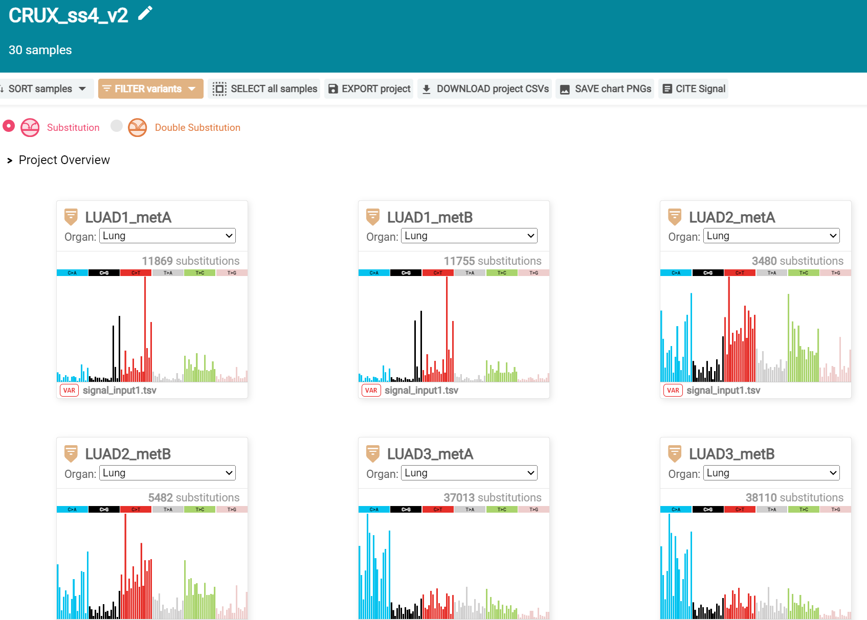
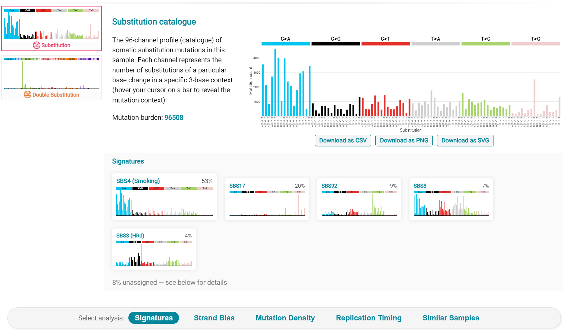
Here we are interested in tumours LUAD1_metA and LUAD7 primary1 used in the El-Kamand et al manuscript. Clicking on the LUAD1_metA panel brings a number of plots describing single nucleotide variants (SNV) types and frequencies, and the proportion of COSMIC V23 signal seen in the variant complement of this tumour. The first data shown is the Substitution catalogue, the pattern of nucleotide substitutions in this tumour; this is shown in screenshot 27.
Screenshot 27
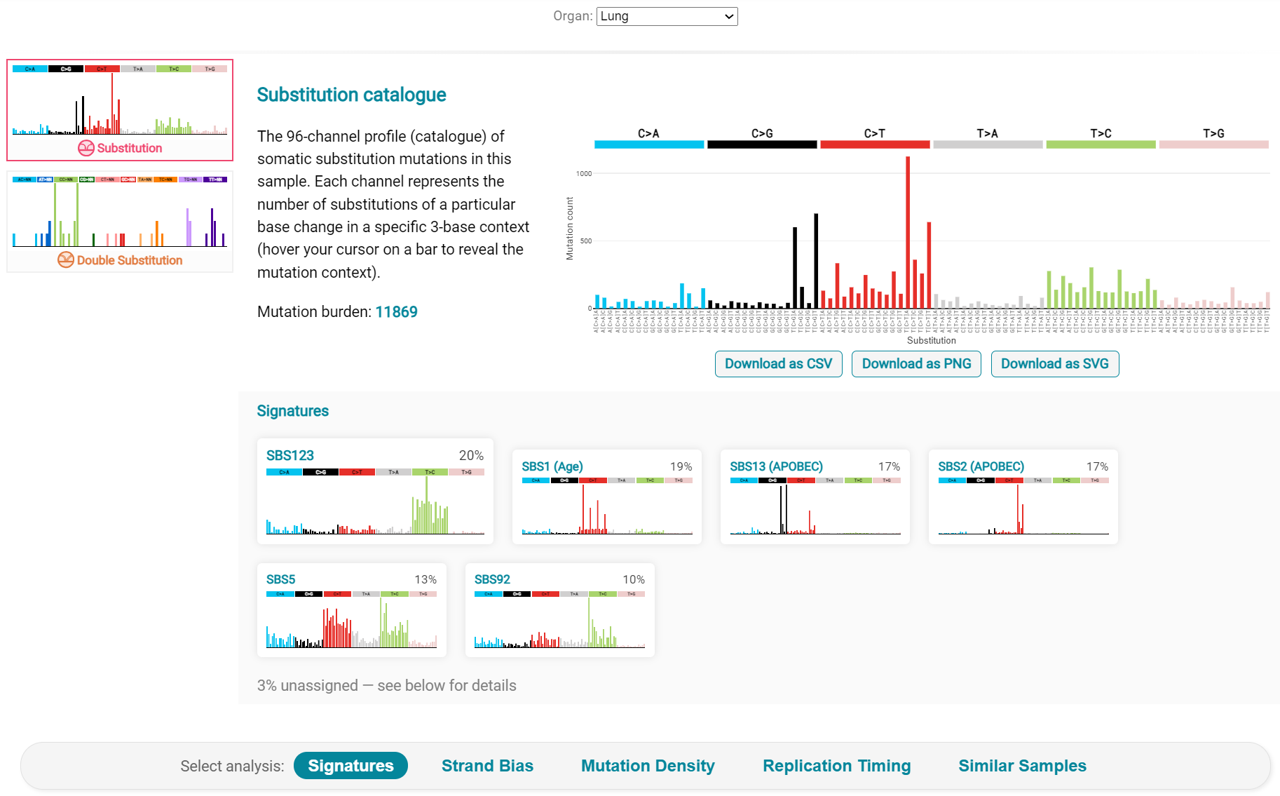
There are a number of analyses we can perform from this page, listed at the bottom, including strand bias, mutation density, replication timing and similar samples. For each there is a text hyperlink at the bottom of the page leading to the relevant page.
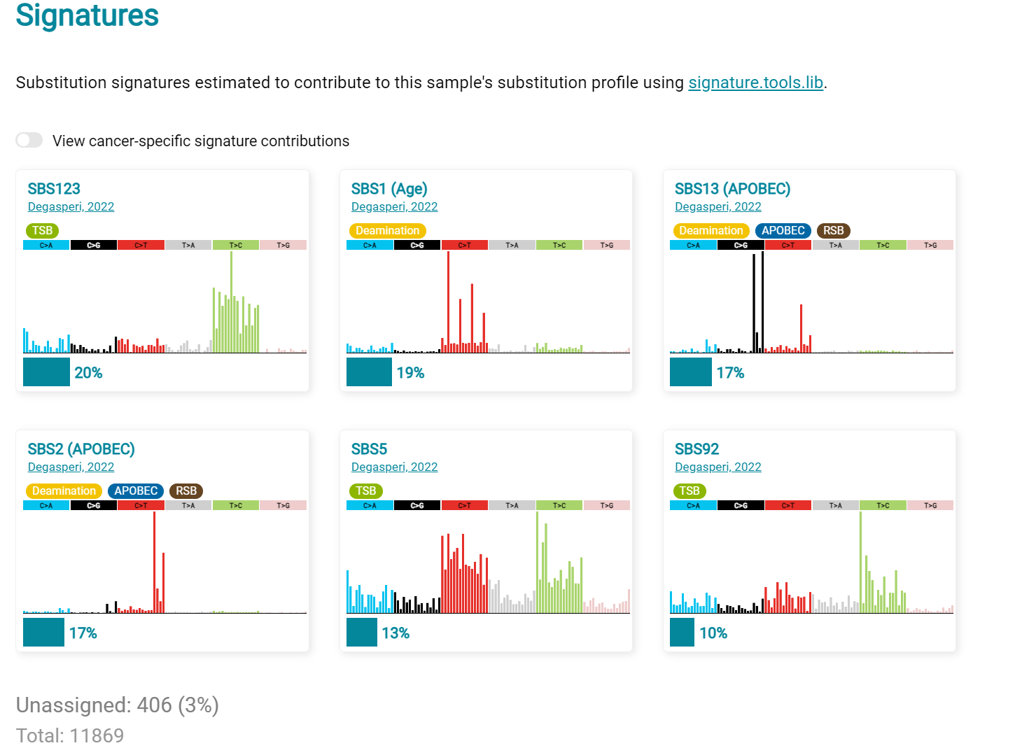
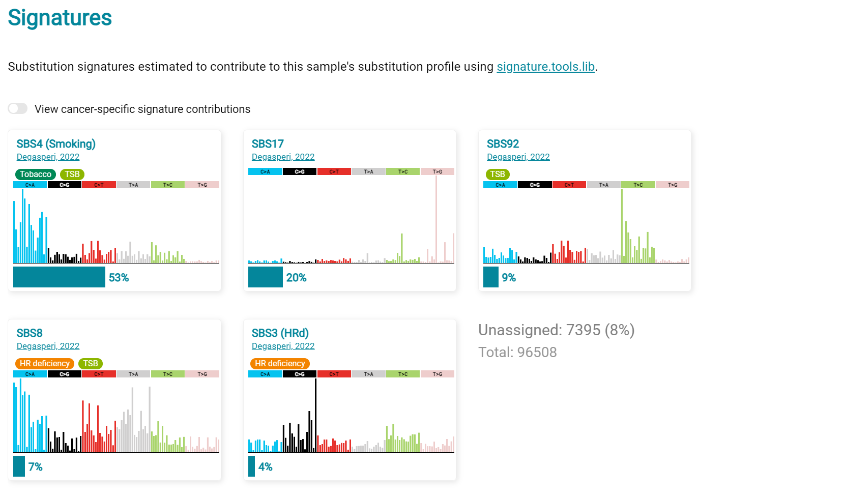
The Signatures analysis shows the relative preponderance of defined COSMIC V3 signatures detected in the sample mutations [screenshot 28]; note that there are a range of other related visualisation provided on this page.
Screenshot 28
The Similar Samples analysis is of particular interest as it can indicate which type of tumours (available to this database) most resemble the mutation patterns seen in this LUAD1 tumour. Screenshot 29 shows the Similar Samples data page.
Screenshot 29
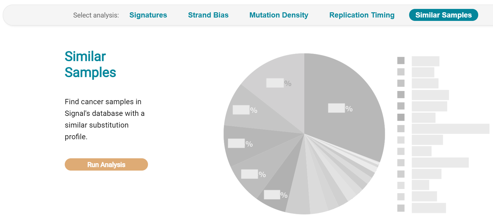
Screenshot 30 shows the output when the analysis is run. The analysis is run with a cosine threshold of 0.96 – the pie chart is similar to that .. container:: example-box
used in the El-Kamand manuscript figure 5D
Screenshot 30
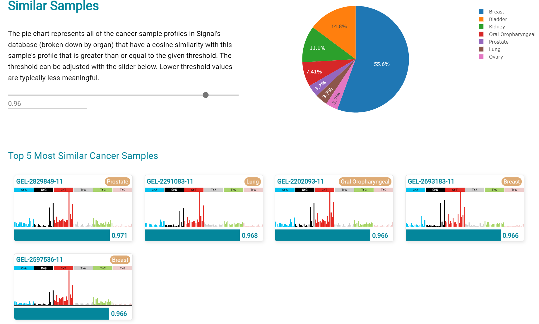
This signature data suggests that the cancer LUAD1 has a pattern of variant that most closely resembles that of Breast Cancer, and only poorly matches Lung cancers.
Next is the analysis of the LUAD7_primary1 tumour, first showing the substitution catalogue which can be seen to be very different to the LUAD7 tumour [screenshot 31].
Screenshot 31
LUAD7 sample Signatures analysis (COSMIC V3 signatures) in this sample is shown in screenshot 32. Note the prominent SBS4 smoking associated signature, absent in LUAD1.
Screenshot 32
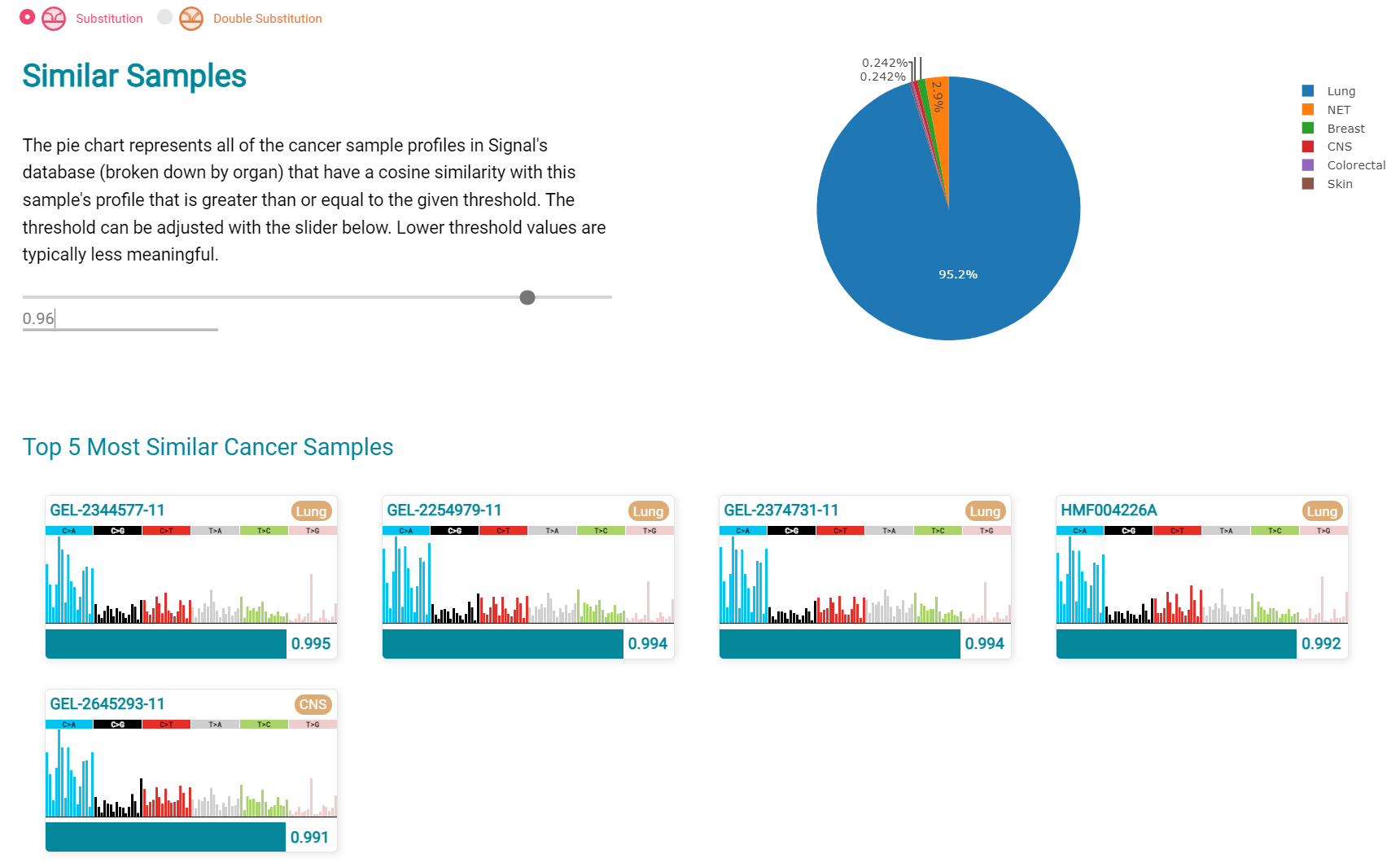
The Similar Sample analysis of LUAD7 sample greatly resembles Lung cancers, unlike (again) LUAD1 [screenshot 33]. This may reflect a preponderance of lung cancers in the Signal database that are caused by smoking.
Screenshot 33
Short study 5: Comparing Virtual Cohorts
Gene mutations associated with triple-negative breast cancer.
Dataset: The TCGA Breast Invasive Carcinoma cohort dataset (n = 978) including ductal and lobular carcinomas. The dataset is provided in CRUX, with one modification: triple negative breast carcinoma samples are labelled (under clinical feature ‘triple-negative_ER_PR_HER2_status’) for demonstration purposes, but this subset can easily be constructed using subset and merge functions under the utilities menu in the sidebar.
In this study we compare triple negative breast cancers (TNBC) against the not-triple negative breast cancers (designated ‘not_TNBC’) to identify mutations associated with these subtypes. Since this TCGA dataset contains samples from male breast cancers these are first filtered out, then then the sub-cohorts are constructed using the ‘subset’ utility; these two subtypes are then using the ‘Compare cohorts’ function on the CRUX sidebar.
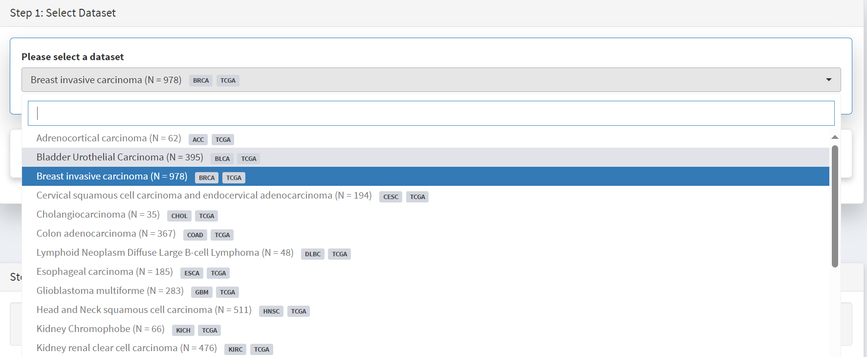
Under Utilities (CRUX sidebar) there is access to the Subset page [screenshot 1]. The page has several panels to work through. First, on Step 1 panel, clicking on the field will cause the available datasets menu to drop down; the Breast Invasive Carcinoma dataset is then selected.
Screenshot 1
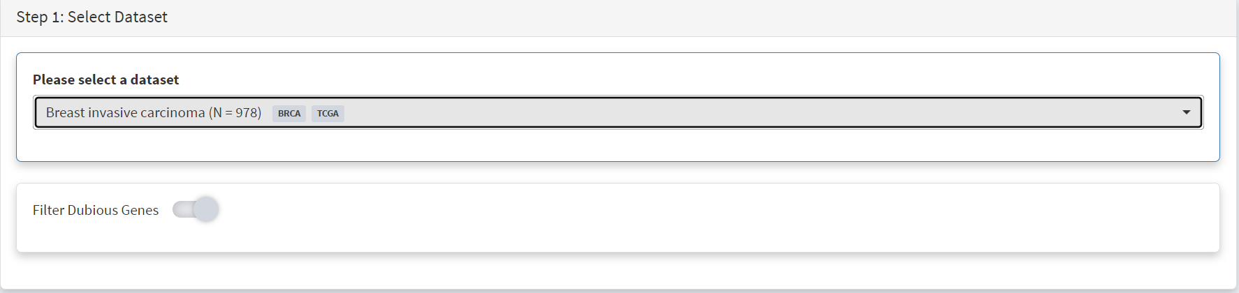
We then filter out ‘dubious genes’ (which commonly carry passenger mutations) on the lower panel section [screenshot 2].
Screenshot 2
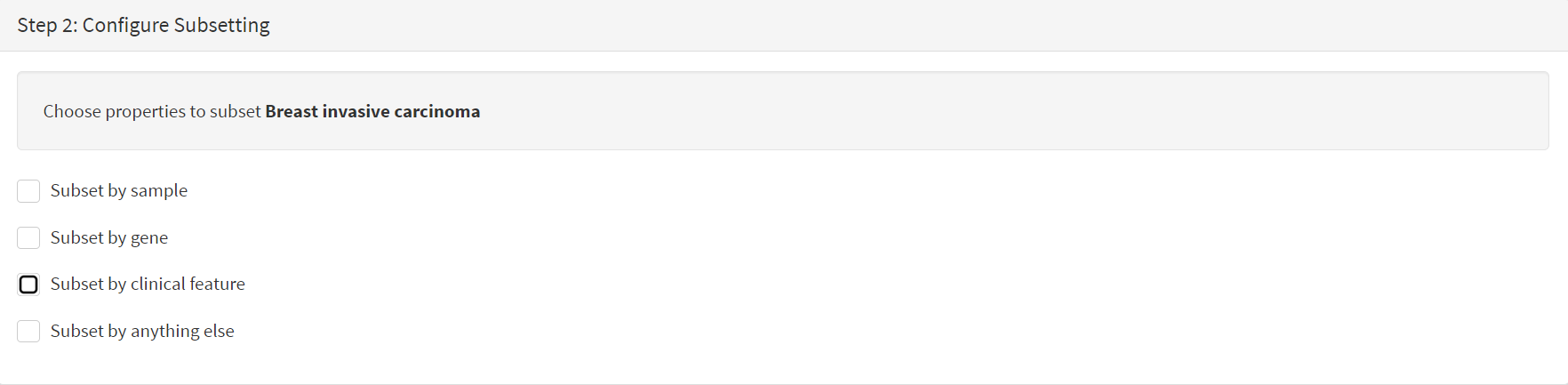
Then in Step 2 panel for our purposes we need to subset the data using a clinical feature [screenshot 3].
Screenshot 3
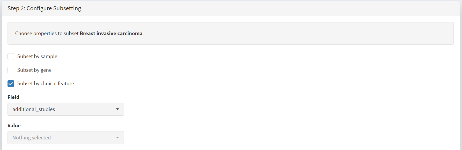
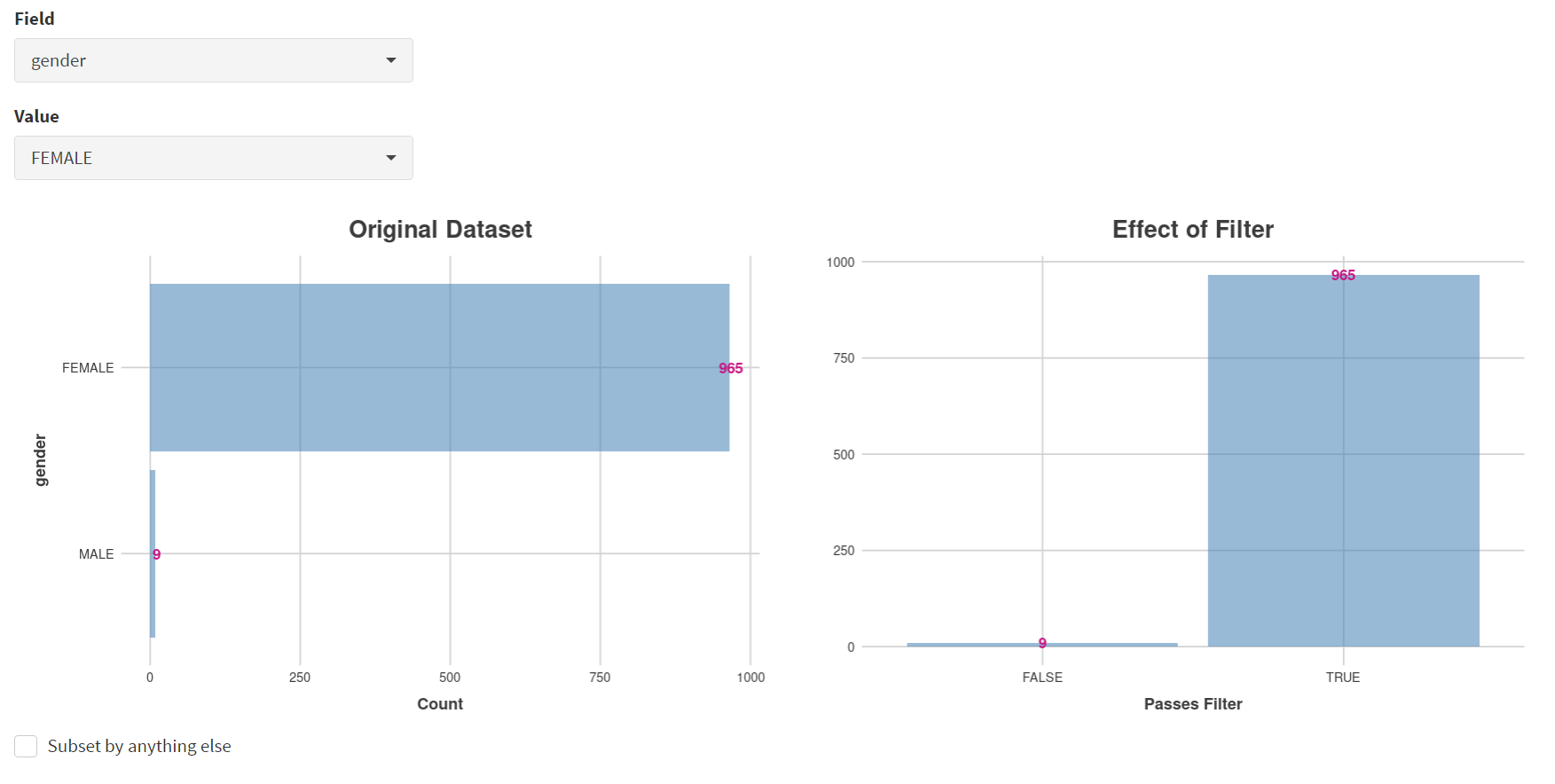
When clinical feature is checked, Field and Value menus become available [screenshot 4]. These are drop down menus containing features available to the user.
Screenshot 4
Male breast cancer cases will be excluded here, so Field = ‘gender’ and Value = ‘FEMALE’ are selected. These immediately give plots showing the size of the subtypes [screenshot 5]; 966 famales and 9 males are shown.
Screenshot 5
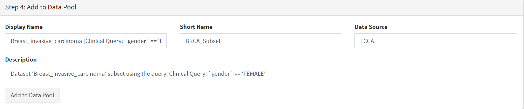
These female-only category needs to be named and entered as a CRUX dataset for further use. This is shown in the Step 6 panel [screenshots 6 and 7].
Screenshot 6
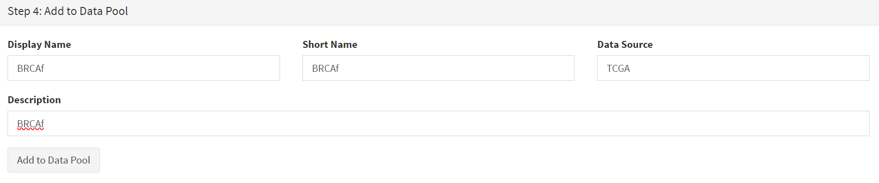
We simply name these ‘BRCAf’ [screenshot 7].
Screenshot 7
Pressing the Add to Data Pool button beneath the fields brings pop-up confirmation that the dataset has been imported [screenshot 8].
Screenshot 8

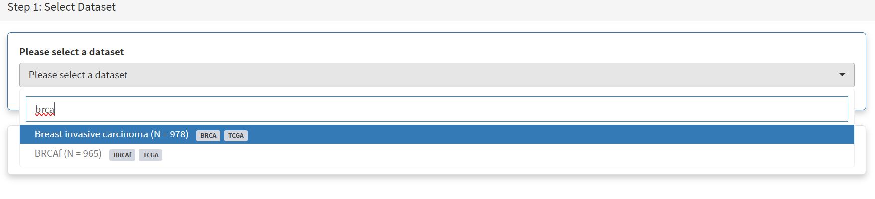
Returning to the top of the page to perform the second subsetting, typing ‘brca’ in the selection field [screenshot 9] brings up the original dataset (highlighted) but also the BRCAf dataset below it. Note that the dataset is available but not saved for future use, so that if CRUX is exited, it will need to be recreated to use.
Screenshot 9
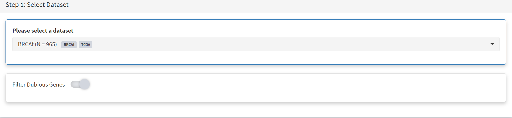
BRCAf is then selected, and Filter Dubious Genes turned on [screenshot 10].
Screenshot 10
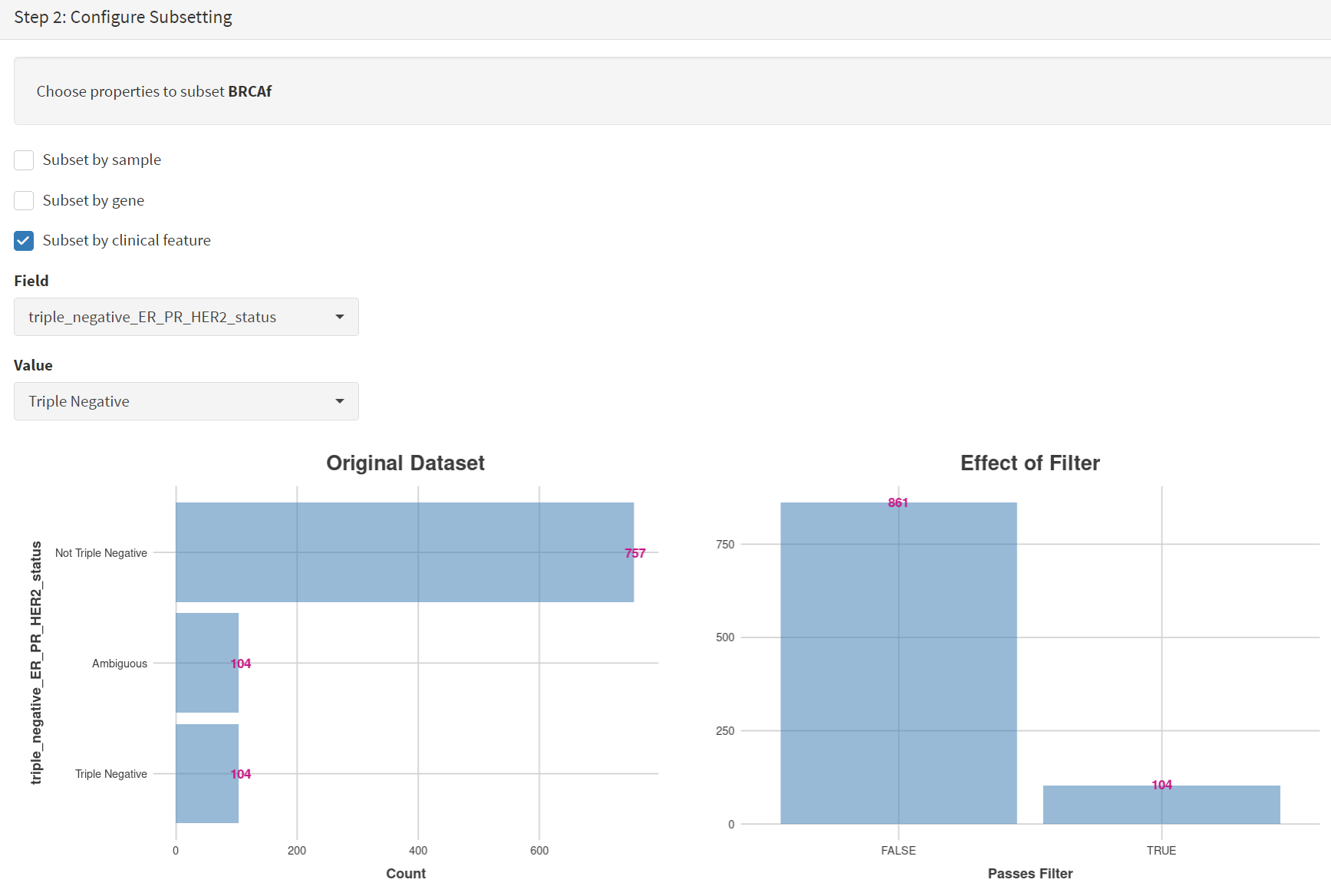
Next the subsetting of BRCAf is configured using Field= ‘triple_negative_ER-PR_HER2_subtype’ and Value = ‘Not Triple Negative’ [screenshot 11]. Note this subtype field was added to the dataset for this study, but in the manuscript work was created using the individual clinical features:
Field= ‘breast_carcinoma_estrogen_receptor_status’, Value= Positive’, OR
Field= ‘breast_carcinoma_progesterone_receptor_status’, Value= Positive’ OR
Field= ‘lab_proc_her2_neu_immunohistochemistry_receptor_status’, Value= Positive’.
These subsets were merged using the CRUX ‘merge’ Utility, equivalent to OR function.
Screenshot 11
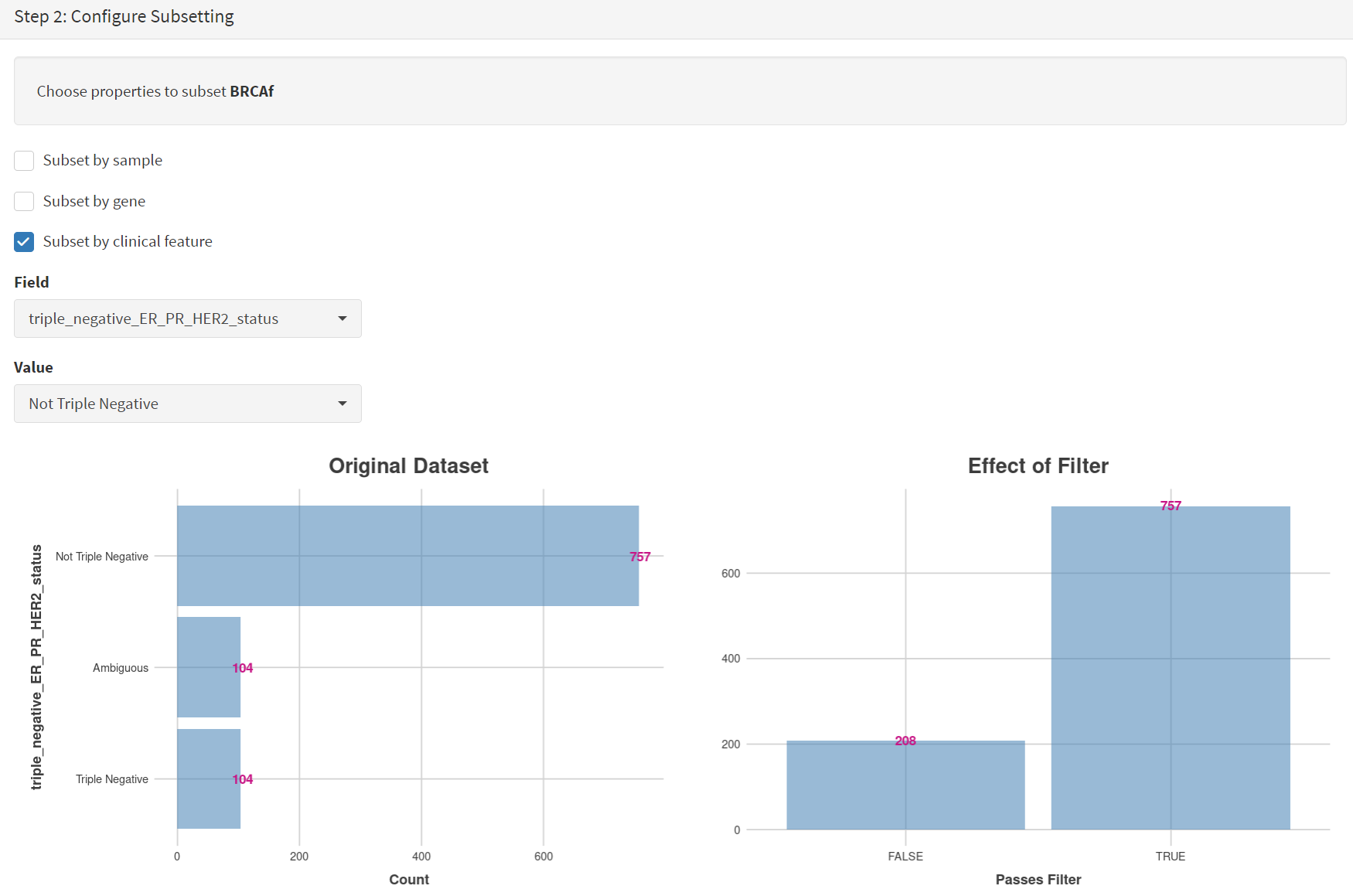
Note that only one subset at a time is created using this subset utility. This is because there are often cancer samples with intermediate (above, Ambiguous) and undocumented (‘NA’) Values that we usually wish to ignore or analyse separately. For many of the Values, if it is required to include more that one Value of cancer, more than on can be selected. Also note that since there may be missing Clinical Feature fields for some samples, the number of cancer samples in the subtypes may sum to less that total samples in the dataset.
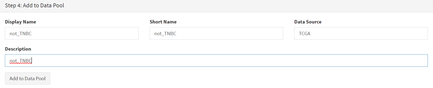
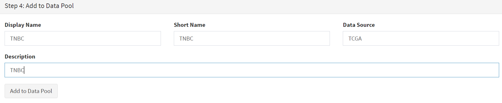
This subset needs to be given a name (we ues ‘not_TNBC’ here) in the Step 4 panel [screenshot 12] and the Add to Dataset button pressed. The pop up alert (not shown) confirms the sub-cohort is available.
Screenshot 12
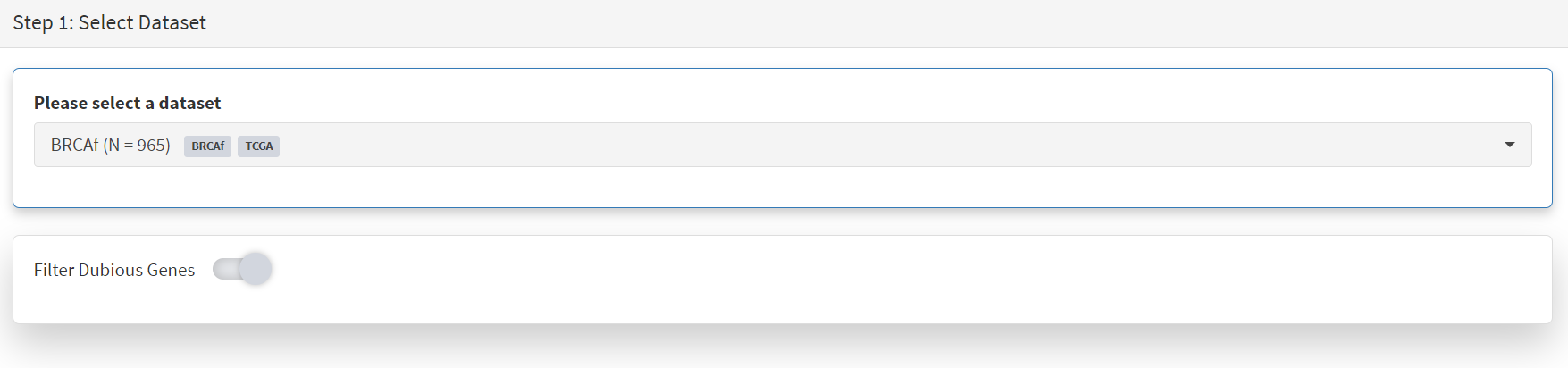
Then, the process is repeated to create the triple negative dataset (TNBC) from the samples in the BRCAf set, starting at the first panel [screenshot 13].
Screenshot 13
The subsetting is repeated as before, using using Field= ‘triple_negative_ER-PR_HER2_subtype’ and Value = ‘Triple Negative’ [screenshot 14]. In the manuscript work we employed:
Field= ‘breast_carcinoma_estrogen_receptor_status’, Value= Negative, AND
Field= ‘breast_carcinoma_progesterone_receptor_status’, Value= Positive’ AND
Field= ‘lab_proc_her2_neu_immunohistochemistry_receptor_status’, Value= Positive’.
These subsets were sequentially subsetted using the CRUX ‘subset’ Utility, which gives the same result as an AND function.
Screenshot 14
Then giving the subset a name [screenshot 15] and add to the Data pool.
Screenshot 15
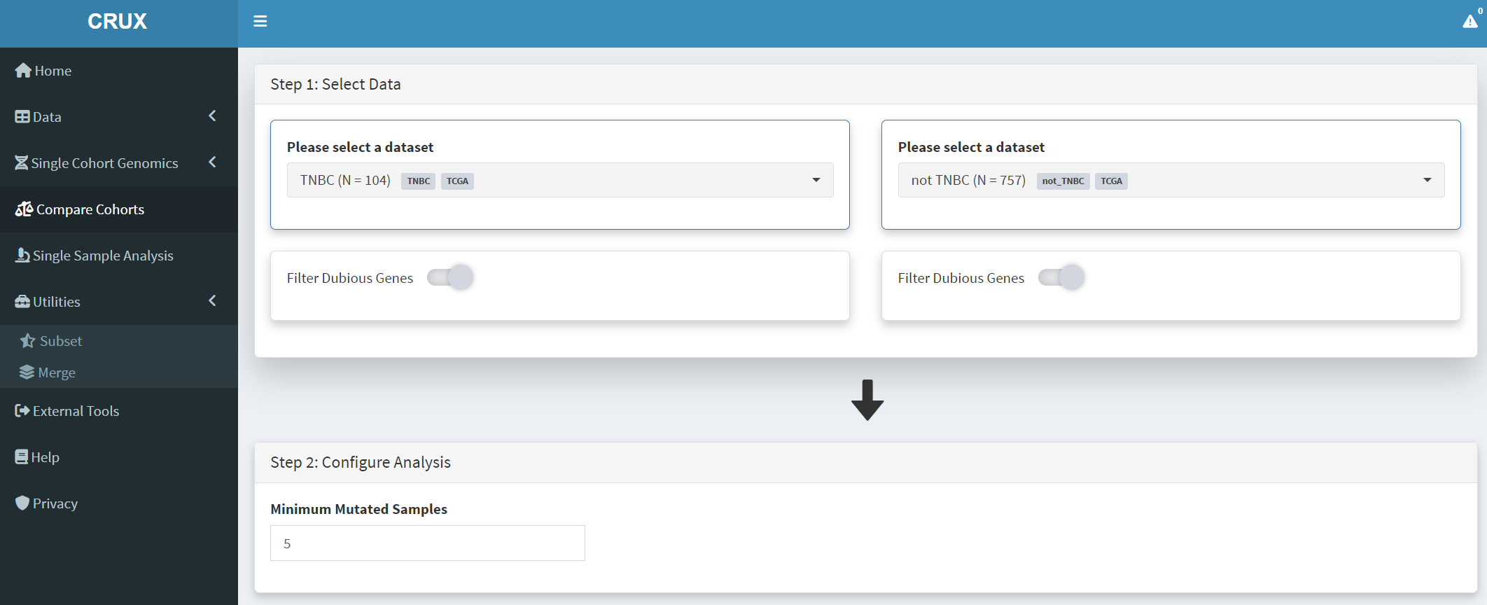
Subsets not_TBBC and TNBC can then be compared with the Compare Cohorts function in the sidebar [screenshot 16].
Screenshot 16
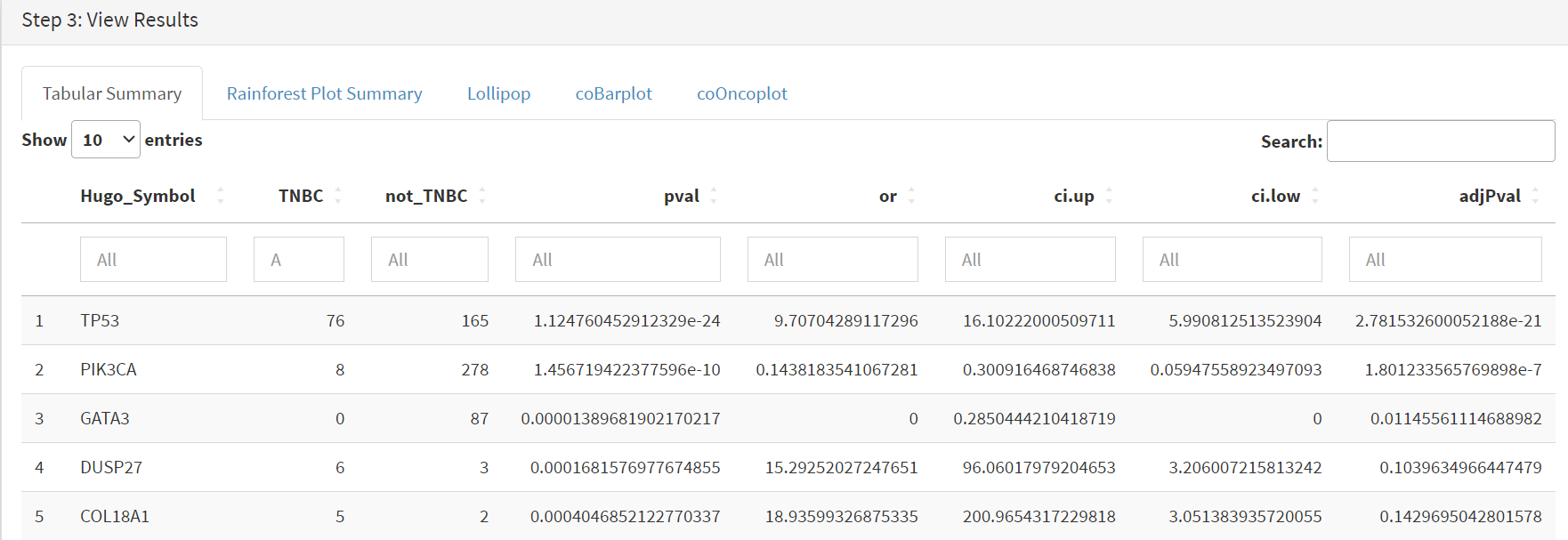
Comparison data is obtained using the Step 3 panel, first a tabular summary [screenshot 17]; top of table only is shown.
Screenshot 17
The next data to view is on the Rainforest Plot Summary tab [screenshot 18] Note that the data is provided as an odds ratio; until recently these tools returned log odds ratio. This screenshot is shown with the FDR < 0.05 selection of the genes of interest. Note P-value column ‘***’ indicates a p-value <0.001.
Screenshot 18
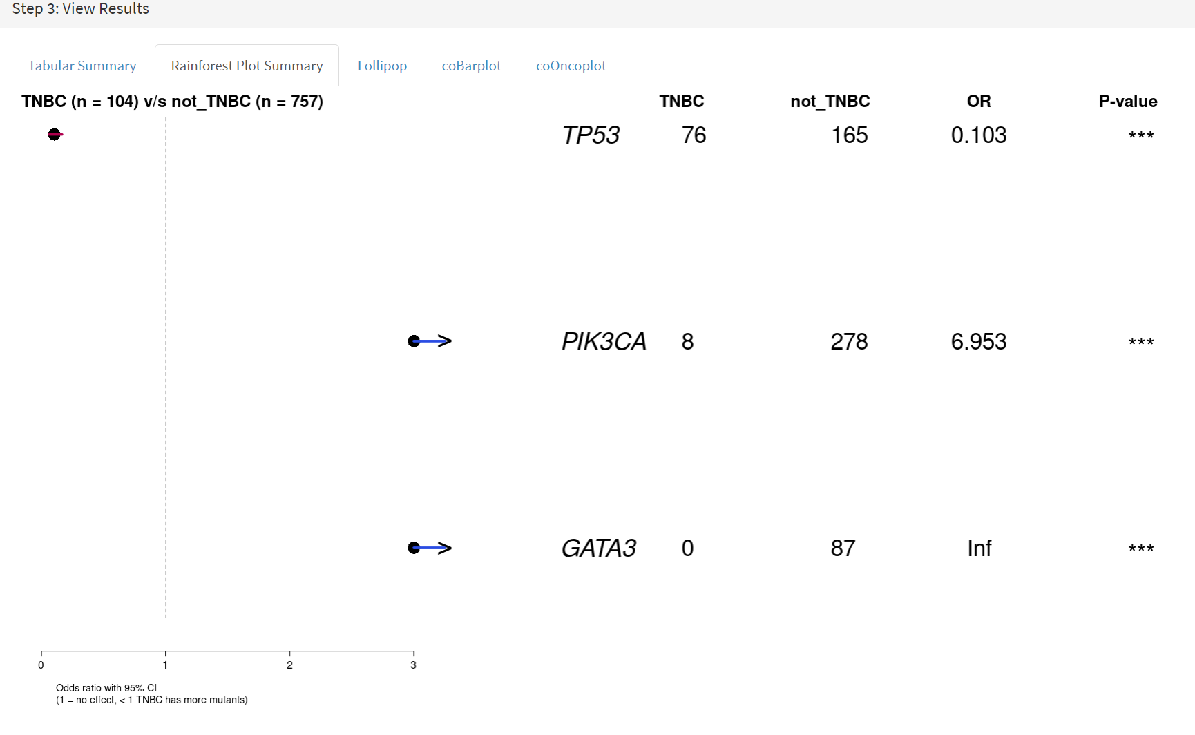
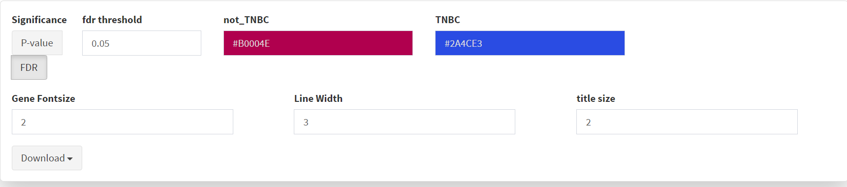
Selection of significant threshold is shown in screenshot 19.
Screenshot 19
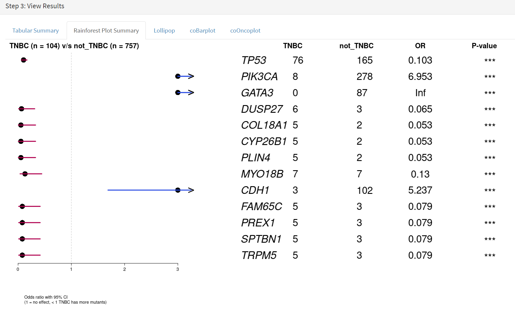
If we select threshold of p-value of 0.001 (not FDR), the results are shown in screenshot 20.
Screenshot 20
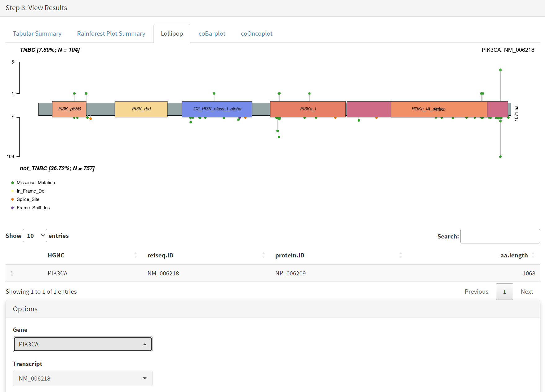
The mutations of a specific gene can be compared between TNBC and not_TNBC sub-cohorts [screenshot 20] in the Lollipop tab; gene PIK3CA is selected from the drop down menu below.
Screenshot 20
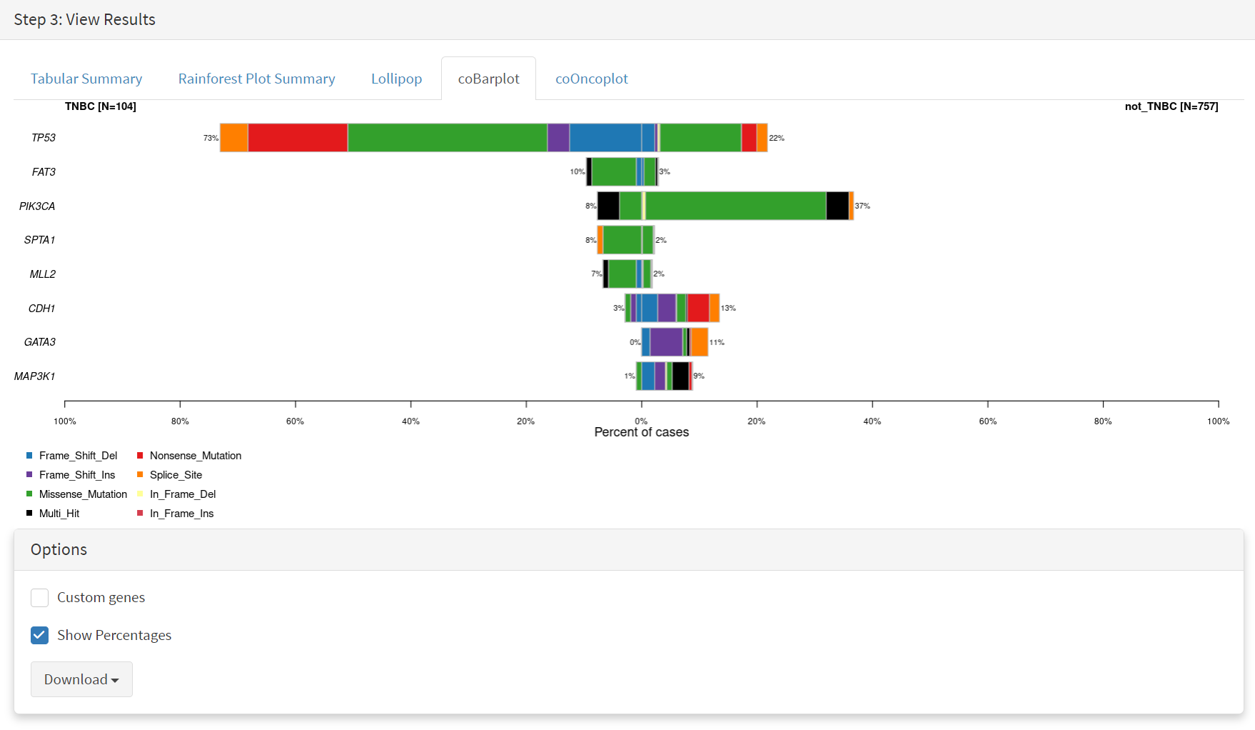
The coBarplot tab gives a comparison of gene mutation frequencies [screenshot 21]. Here, the TNBC frequencies go to the left and not_TNBC go to the right, ie.e., showing two horizontal plots both with ‘0%’ as the baseline. The types of mutations are indicated by colour bands, with the key below the plot. This plot can be downloaded using the button below.
Screenshot 21
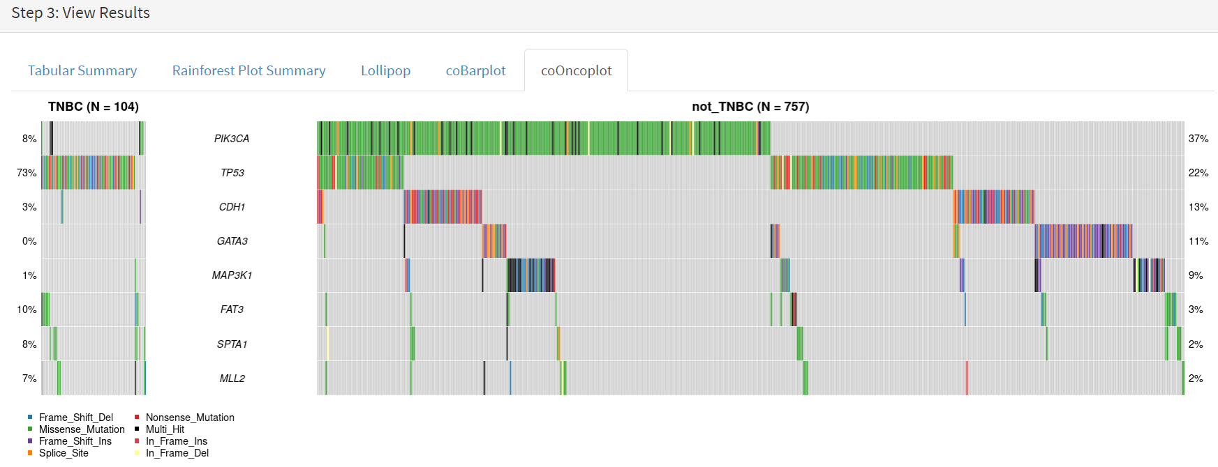
Lastly, side by side oncoplots are shown on the coOncoplot tab [screenshot 22]. The samples are on the X-axis but ordered according mutation occurrence and co-occurrence frequencies. Note that the not_TNBC plot is wider as it contains far more samples.
Screenshot 22